Polynomial Regression Extrapolation [LuxAlgo]

30 thg 6, 2022

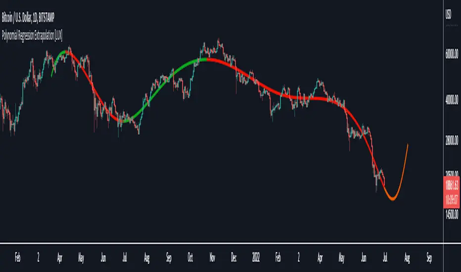
This indicator fits a polynomial with a user set degree to the price using least squares and then extrapolates the result.

Settings

• Length: Number of most recent price observations used to fit the model.
  
• Extrapolate: Extrapolation horizon
  
• Degree: Degree of the fitted polynomial
  
• Src: Input source
  
• Lock Fit: By default the fit and extrapolated result will readjust to any new price observation, enabling this setting allow the model to ignore new price observations, and extend the extrapolation to the most recent bar.
  

Usage

Polynomial regression is commonly used when a relationship between two variables can be described by a polynomial.

In technical analysis polynomial regression is commonly used to estimate underlying trends in the price as well as obtaining support/resistances. One common example being the linear regression which can be described as polynomial regression of degree 1.

Using polynomial regression for extrapolation can be considered when we assume that the underlying trend of a certain asset follows polynomial of a certain degree and that this assumption hold true for time t+1...,t+n. This is rarely the case but it can be of interest to certain users performing longer term analysis of assets such as Bitcoin.

The selection of the polynomial degree can be done considering the underlying trend of the observations we are trying to fit. In practice, it is rare to go over a degree of 3, as higher degree would tend to highlight more noisy variations.



Using a polynomial of degree 1 will return a line, and as such can be considered when the underlying trend is linear, but one could improve the fit by using an higher degree.



The chart above fits a polynomial of degree 2, this can be used to model more parabolic observations. We can see in the chart above that this improves the fit.



In the chart above a polynomial of degree 6 is used, we can see how more variations are highlighted. The extrapolation of higher degree polynomials can eventually highlight future turning points due to the nature of the polynomial, however there are no guarantee that these will reflect exact future reversals.

Details

A polynomial regression model y(t) of degree p is described by:

y(t) = β(0) + β(1)x(t) + β(2)x(t)^2 + ... + β(p)x(t)^p

The vector coefficients β are obtained such that the sum of squared error between the observations and y(t) is minimized. This can be achieved through specific iterative algorithms or directly by solving the system of equations:

β(0) + β(1)x(0) + β(2)x(0)^2 + ... + β(p)x(0)^p = y(0)β(0) + β(1)x(1) + β(2)x(1)^2 + ... + β(p)x(1)^p = y(1)...β(0) + β(1)x(t-1) + β(2)x(t-1)^2 + ... + β(p)x(t-1)^p = y(t-1)Note that solving this system of equations for higher degrees p with high x values can drastically affect the accuracy of the results. One method to circumvent this can be to subtract x by its mean.

5 thg 10, 2022

Phát hành các Ghi chú

Minor changes.