OPEN-SOURCE SCRIPT
Ehlers Phasor Analysis (PHASOR)
# PHASOR: Phasor Analysis (Ehlers)
## Overview and Purpose
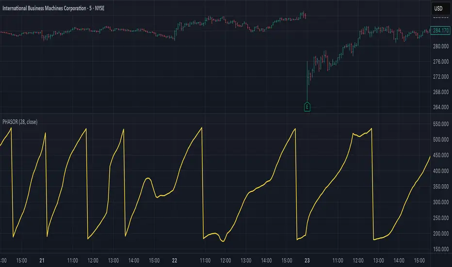
The Phasor Analysis indicator, developed by John Ehlers, represents an advanced cycle analysis tool that identifies the phase of the dominant cycle component in a time series through complex signal processing techniques. This sophisticated indicator uses correlation-based methods to determine the real and imaginary components of the signal, converting them to a continuous phase angle that reveals market cycle progression. Unlike traditional oscillators, the Phasor provides unwrapped phase measurements that accumulate continuously, offering unique insights into market timing and cycle behavior.
## Core Concepts
* **Complex Signal Analysis** — Uses real and imaginary components to determine cycle phase
* **Correlation-Based Detection** — Employs Ehlers' correlation method for robust phase estimation
* **Unwrapped Phase Tracking** — Provides continuous phase accumulation without discontinuities
* **Anti-Regression Logic** — Prevents phase angle from moving backward under specific conditions
Market Applications:
* **Cycle Timing** — Precise identification of cycle peaks and troughs
* **Market Regime Analysis** — Distinguishes between trending and cycling market conditions
* **Turning Point Detection** — Advanced warning system for potential market reversals
## Common Settings and Parameters
| Parameter | Default | Function | When to Adjust |
|-----------|---------|----------|----------------|
| Period | 28 | Fixed cycle period for correlation analysis | Match to expected dominant cycle length |
| Source | Close | Price series for phase calculation | Use typical price or other smoothed series |
| Show Derived Period | false | Display calculated period from phase rate | Enable for adaptive period analysis |
| Show Trend State | false | Display trend/cycle state variable | Enable for regime identification |
## Calculation and Mathematical Foundation
**Technical Formula:**
**Stage 1: Correlation Analysis**
For period $n$ and source $x_t$:
Real component correlation with cosine wave:
$$R = \frac{n \sum x_t \cos\left(\frac{2\pi t}{n}\right) - \sum x_t \sum \cos\left(\frac{2\pi t}{n}\right)}{\sqrt{D_{cos}}}$$
Imaginary component correlation with negative sine wave:
$$I = \frac{n \sum x_t \left(-\sin\left(\frac{2\pi t}{n}\right)\right) - \sum x_t \sum \left(-\sin\left(\frac{2\pi t}{n}\right)\right)}{\sqrt{D_{sin}}}$$
where $D_{cos}$ and $D_{sin}$ are normalization denominators.
**Stage 2: Phase Angle Conversion**
$$\theta_{raw} = \begin{cases}
90° - \arctan\left(\frac{I}{R}\right) \cdot \frac{180°}{\pi} & \text{if } R \neq 0 \\
0° & \text{if } R = 0, I > 0 \\
180° & \text{if } R = 0, I \leq 0
\end{cases}$$
**Stage 3: Phase Unwrapping**
$$\theta_{unwrapped}(t) = \theta_{unwrapped}(t-1) + \Delta\theta$$
where $\Delta\theta$ is the normalized phase difference.
**Stage 4: Ehlers' Anti-Regression Condition**
$$\theta_{final}(t) = \begin{cases}
\theta_{final}(t-1) & \text{if regression conditions met} \\
\theta_{unwrapped}(t) & \text{otherwise}
\end{cases}$$
**Derived Calculations:**
Derived Period: $P_{derived} = \frac{360°}{\Delta\theta_{final}}$ (clamped to [1, 60])
Trend State:
$$S_{trend} = \begin{cases}
1 & \text{if } \Delta\theta \leq 6° \text{ and } |\theta| \geq 90° \\
-1 & \text{if } \Delta\theta \leq 6° \text{ and } |\theta| < 90° \\
0 & \text{if } \Delta\theta > 6°
\end{cases}$$
> 🔍 **Technical Note:** The correlation-based approach provides robust phase estimation even in noisy market conditions, while the unwrapping mechanism ensures continuous phase tracking across cycle boundaries.
## Interpretation Details
* **Phasor Angle (Primary Output):**
- **+90°**: Potential cycle peak region
- **0°**: Mid-cycle ascending phase
- **-90°**: Potential cycle trough region
- **±180°**: Mid-cycle descending phase
* **Phase Progression:**
- Continuous upward movement → Normal cycle progression
- Phase stalling → Potential cycle extension or trend development
- Rapid phase changes → Cycle compression or volatility spike
* **Derived Period Analysis:**
- Period < 10 → High-frequency cycle dominance
- Period 15-40 → Typical swing trading cycles
- Period > 50 → Trending market conditions
* **Trend State Variable:**
- **+1**: Long trend conditions (slow phase change in extreme zones)
- **-1**: Short trend or consolidation (slow phase change in neutral zones)
- **0**: Active cycling (normal phase change rate)
## Applications
* **Cycle-Based Trading:**
- Enter long positions near -90° crossings (cycle troughs)
- Enter short positions near +90° crossings (cycle peaks)
- Exit positions during mid-cycle phases (0°, ±180°)
* **Market Timing:**
- Use phase acceleration for early trend detection
- Monitor derived period for cycle length changes
- Combine with trend state for regime-appropriate strategies
* **Risk Management:**
- Adjust position sizes based on cycle clarity (derived period stability)
- Implement different risk parameters for trending vs. cycling regimes
- Use phase velocity for stop-loss placement timing
## Limitations and Considerations
* **Parameter Sensitivity:**
- Fixed period assumption may not match actual market cycles
- Requires cycle period optimization for different markets and timeframes
- Performance degrades when multiple cycles interfere
* **Computational Complexity:**
- Correlation calculations over full period windows
- Multiple mathematical transformations increase processing requirements
- Real-time implementation requires efficient algorithms
* **Market Conditions:**
- Most effective in markets with clear cyclical behavior
- May provide false signals during strong trending periods
- Requires sufficient historical data for correlation analysis
Complementary Indicators:
* MESA Adaptive Moving Average (cycle-based smoothing)
* Dominant Cycle Period indicators
* Detrended Price Oscillator (cycle identification)
## References
1. Ehlers, J.F. "Cycle Analytics for Traders." Wiley, 2013.
2. Ehlers, J.F. "Cybernetic Analysis for Stocks and Futures." Wiley, 2004.
## Overview and Purpose
The Phasor Analysis indicator, developed by John Ehlers, represents an advanced cycle analysis tool that identifies the phase of the dominant cycle component in a time series through complex signal processing techniques. This sophisticated indicator uses correlation-based methods to determine the real and imaginary components of the signal, converting them to a continuous phase angle that reveals market cycle progression. Unlike traditional oscillators, the Phasor provides unwrapped phase measurements that accumulate continuously, offering unique insights into market timing and cycle behavior.
## Core Concepts
* **Complex Signal Analysis** — Uses real and imaginary components to determine cycle phase
* **Correlation-Based Detection** — Employs Ehlers' correlation method for robust phase estimation
* **Unwrapped Phase Tracking** — Provides continuous phase accumulation without discontinuities
* **Anti-Regression Logic** — Prevents phase angle from moving backward under specific conditions
Market Applications:
* **Cycle Timing** — Precise identification of cycle peaks and troughs
* **Market Regime Analysis** — Distinguishes between trending and cycling market conditions
* **Turning Point Detection** — Advanced warning system for potential market reversals
## Common Settings and Parameters
| Parameter | Default | Function | When to Adjust |
|-----------|---------|----------|----------------|
| Period | 28 | Fixed cycle period for correlation analysis | Match to expected dominant cycle length |
| Source | Close | Price series for phase calculation | Use typical price or other smoothed series |
| Show Derived Period | false | Display calculated period from phase rate | Enable for adaptive period analysis |
| Show Trend State | false | Display trend/cycle state variable | Enable for regime identification |
## Calculation and Mathematical Foundation
**Technical Formula:**
**Stage 1: Correlation Analysis**
For period $n$ and source $x_t$:
Real component correlation with cosine wave:
$$R = \frac{n \sum x_t \cos\left(\frac{2\pi t}{n}\right) - \sum x_t \sum \cos\left(\frac{2\pi t}{n}\right)}{\sqrt{D_{cos}}}$$
Imaginary component correlation with negative sine wave:
$$I = \frac{n \sum x_t \left(-\sin\left(\frac{2\pi t}{n}\right)\right) - \sum x_t \sum \left(-\sin\left(\frac{2\pi t}{n}\right)\right)}{\sqrt{D_{sin}}}$$
where $D_{cos}$ and $D_{sin}$ are normalization denominators.
**Stage 2: Phase Angle Conversion**
$$\theta_{raw} = \begin{cases}
90° - \arctan\left(\frac{I}{R}\right) \cdot \frac{180°}{\pi} & \text{if } R \neq 0 \\
0° & \text{if } R = 0, I > 0 \\
180° & \text{if } R = 0, I \leq 0
\end{cases}$$
**Stage 3: Phase Unwrapping**
$$\theta_{unwrapped}(t) = \theta_{unwrapped}(t-1) + \Delta\theta$$
where $\Delta\theta$ is the normalized phase difference.
**Stage 4: Ehlers' Anti-Regression Condition**
$$\theta_{final}(t) = \begin{cases}
\theta_{final}(t-1) & \text{if regression conditions met} \\
\theta_{unwrapped}(t) & \text{otherwise}
\end{cases}$$
**Derived Calculations:**
Derived Period: $P_{derived} = \frac{360°}{\Delta\theta_{final}}$ (clamped to [1, 60])
Trend State:
$$S_{trend} = \begin{cases}
1 & \text{if } \Delta\theta \leq 6° \text{ and } |\theta| \geq 90° \\
-1 & \text{if } \Delta\theta \leq 6° \text{ and } |\theta| < 90° \\
0 & \text{if } \Delta\theta > 6°
\end{cases}$$
> 🔍 **Technical Note:** The correlation-based approach provides robust phase estimation even in noisy market conditions, while the unwrapping mechanism ensures continuous phase tracking across cycle boundaries.
## Interpretation Details
* **Phasor Angle (Primary Output):**
- **+90°**: Potential cycle peak region
- **0°**: Mid-cycle ascending phase
- **-90°**: Potential cycle trough region
- **±180°**: Mid-cycle descending phase
* **Phase Progression:**
- Continuous upward movement → Normal cycle progression
- Phase stalling → Potential cycle extension or trend development
- Rapid phase changes → Cycle compression or volatility spike
* **Derived Period Analysis:**
- Period < 10 → High-frequency cycle dominance
- Period 15-40 → Typical swing trading cycles
- Period > 50 → Trending market conditions
* **Trend State Variable:**
- **+1**: Long trend conditions (slow phase change in extreme zones)
- **-1**: Short trend or consolidation (slow phase change in neutral zones)
- **0**: Active cycling (normal phase change rate)
## Applications
* **Cycle-Based Trading:**
- Enter long positions near -90° crossings (cycle troughs)
- Enter short positions near +90° crossings (cycle peaks)
- Exit positions during mid-cycle phases (0°, ±180°)
* **Market Timing:**
- Use phase acceleration for early trend detection
- Monitor derived period for cycle length changes
- Combine with trend state for regime-appropriate strategies
* **Risk Management:**
- Adjust position sizes based on cycle clarity (derived period stability)
- Implement different risk parameters for trending vs. cycling regimes
- Use phase velocity for stop-loss placement timing
## Limitations and Considerations
* **Parameter Sensitivity:**
- Fixed period assumption may not match actual market cycles
- Requires cycle period optimization for different markets and timeframes
- Performance degrades when multiple cycles interfere
* **Computational Complexity:**
- Correlation calculations over full period windows
- Multiple mathematical transformations increase processing requirements
- Real-time implementation requires efficient algorithms
* **Market Conditions:**
- Most effective in markets with clear cyclical behavior
- May provide false signals during strong trending periods
- Requires sufficient historical data for correlation analysis
Complementary Indicators:
* MESA Adaptive Moving Average (cycle-based smoothing)
* Dominant Cycle Period indicators
* Detrended Price Oscillator (cycle identification)
## References
1. Ehlers, J.F. "Cycle Analytics for Traders." Wiley, 2013.
2. Ehlers, J.F. "Cybernetic Analysis for Stocks and Futures." Wiley, 2004.
Mã nguồn mở
Theo đúng tinh thần TradingView, tác giả của tập lệnh này đã công bố nó dưới dạng mã nguồn mở, để các nhà giao dịch có thể xem xét và xác minh chức năng. Chúc mừng tác giả! Mặc dù bạn có thể sử dụng miễn phí, hãy nhớ rằng việc công bố lại mã phải tuân theo Nội quy.
github.com/mihakralj/pinescript
A collection of mathematically rigorous technical indicators for Pine Script 6, featuring defensible math, optimized implementations, proper state initialization, and O(1) constant time efficiency where possible.
A collection of mathematically rigorous technical indicators for Pine Script 6, featuring defensible math, optimized implementations, proper state initialization, and O(1) constant time efficiency where possible.
Thông báo miễn trừ trách nhiệm
Thông tin và các ấn phẩm này không nhằm mục đích, và không cấu thành, lời khuyên hoặc khuyến nghị về tài chính, đầu tư, giao dịch hay các loại khác do TradingView cung cấp hoặc xác nhận. Đọc thêm tại Điều khoản Sử dụng.