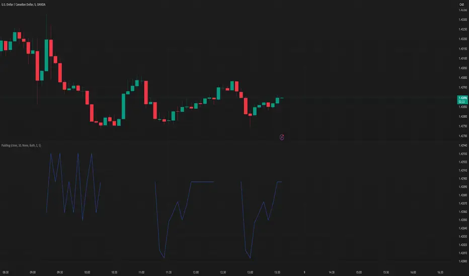
PaddingThe Padding library is a comprehensive and flexible toolkit designed to extend time series data within TradingView, making it an indispensable resource for advanced signal processing tasks such as FFT, filtering, convolution, and wavelet analysis. At its core, the library addresses the common challenge of edge effects by "padding" your data—that is, by appending additional data points beyond the natural boundaries of your original dataset. This extension not only mitigates the distortions that can occur at the endpoints but also helps to maintain the integrity of various transformations and calculations performed on the series. The library accomplishes this while preserving the ordering of your data, ensuring that the most recent point always resides at index 0.
Central to the functionality of this library are two key enumerations: Direction and PaddingType. The Direction enum determines where the padding will be applied. You can choose to extend the data in the forward direction (ahead of the current values), in the backward direction (behind the current values), or in both directions simultaneously. The PaddingType enum defines the specific method used for extending the data. The library supports several methods—including symmetric, reflect, periodic, antisymmetric, antireflect, smooth, constant, and zero padding—each of which has been implemented to suit different analytical scenarios. For instance, symmetric padding mirrors the original data across its boundaries, while reflect padding continues the trend by reflecting around endpoint values. Periodic padding repeats the data, and antisymmetric padding mirrors the data with alternating signs to counterbalance it. The antireflect and smooth methods take into account the derivatives of your data, thereby extending the series in a way that preserves or smoothly continues these derivative values. Constant and zero padding simply extend the series using fixed endpoint values or zeros. Together, these enums allow you to fine-tune how your data is extended, ensuring that the padding method aligns with the specific requirements of your analysis.
The library is designed to work with both single variable inputs and array inputs. When using array-based methods—particularly with the antireflect and smooth padding types—please note that the implementation intentionally discards the last data point as a result of the delta computation process. This behavior is an important consideration when integrating the library into your TradingView studies, as it affects the overall data length of the padded series. Despite this, the library’s structure and documentation make it straightforward to incorporate into your existing scripts. You simply provide your data source, define the length of your data window, and select the desired padding type and direction, along with any optional parameters to control the extent of the padding (using both_period, forward_period, or backward_period).
In practical application, the Padding library enables you to extend historical data beyond its original range in a controlled and predictable manner. This is particularly useful when preparing datasets for further signal processing, as it helps to reduce artifacts that can otherwise compromise the results of your analytical routines. Whether you are an experienced Pine Script developer or a trader exploring advanced data analysis techniques, this library offers a robust solution that enhances the reliability and accuracy of your studies by ensuring your algorithms operate on a more complete and well-prepared dataset.
Library "Padding"
A comprehensive library for padding time series data with various methods. Supports both single variable and array inputs, with flexible padding directions and periods. Designed for signal processing applications including FFT, filtering, convolution, and wavelets. All methods maintain data ordering with most recent point at index 0.
symmetric(source, series_length, direction, both_period, forward_period, backward_period)
Applies symmetric padding by mirroring the input data across boundaries
Parameters:
source (float) : Input value to pad from
series_length (int) : Length of the data window
direction (series Direction) : Direction to apply padding
both_period (int) : Optional - periods to pad in both directions. Overrides forward_period and backward_period if specified
forward_period (int) : Optional - periods to pad forward. Defaults to series_length if not specified
backward_period (int) : Optional - periods to pad backward. Defaults to series_length if not specified
Returns: Array ordered with most recent point at index 0, containing original data with symmetric padding applied
method symmetric(source, direction, both_period, forward_period, backward_period)
Applies symmetric padding to an array by mirroring the data across boundaries
Namespace types: array
Parameters:
source (array) : Array of values to pad
direction (series Direction) : Direction to apply padding
both_period (int) : Optional - periods to pad in both directions. Overrides forward_period and backward_period if specified
forward_period (int) : Optional - periods to pad forward. Defaults to array length if not specified
backward_period (int) : Optional - periods to pad backward. Defaults to array length if not specified
Returns: Array ordered with most recent point at index 0, containing original data with symmetric padding applied
reflect(source, series_length, direction, both_period, forward_period, backward_period)
Applies reflect padding by continuing trends through reflection around endpoint values
Parameters:
source (float) : Input value to pad from
series_length (int) : Length of the data window
direction (series Direction) : Direction to apply padding
both_period (int) : Optional - periods to pad in both directions. Overrides forward_period and backward_period if specified
forward_period (int) : Optional - periods to pad forward. Defaults to series_length if not specified
backward_period (int) : Optional - periods to pad backward. Defaults to series_length if not specified
Returns: Array ordered with most recent point at index 0, containing original data with reflect padding applied
method reflect(source, direction, both_period, forward_period, backward_period)
Applies reflect padding to an array by continuing trends through reflection around endpoint values
Namespace types: array
Parameters:
source (array) : Array of values to pad
direction (series Direction) : Direction to apply padding
both_period (int) : Optional - periods to pad in both directions. Overrides forward_period and backward_period if specified
forward_period (int) : Optional - periods to pad forward. Defaults to array length if not specified
backward_period (int) : Optional - periods to pad backward. Defaults to array length if not specified
Returns: Array ordered with most recent point at index 0, containing original data with reflect padding applied
periodic(source, series_length, direction, both_period, forward_period, backward_period)
Applies periodic padding by repeating the input data
Parameters:
source (float) : Input value to pad from
series_length (int) : Length of the data window
direction (series Direction) : Direction to apply padding
both_period (int) : Optional - periods to pad in both directions. Overrides forward_period and backward_period if specified
forward_period (int) : Optional - periods to pad forward. Defaults to series_length if not specified
backward_period (int) : Optional - periods to pad backward. Defaults to series_length if not specified
Returns: Array ordered with most recent point at index 0, containing original data with periodic padding applied
method periodic(source, direction, both_period, forward_period, backward_period)
Applies periodic padding to an array by repeating the data
Namespace types: array
Parameters:
source (array) : Array of values to pad
direction (series Direction) : Direction to apply padding
both_period (int) : Optional - periods to pad in both directions. Overrides forward_period and backward_period if specified
forward_period (int) : Optional - periods to pad forward. Defaults to array length if not specified
backward_period (int) : Optional - periods to pad backward. Defaults to array length if not specified
Returns: Array ordered with most recent point at index 0, containing original data with periodic padding applied
antisymmetric(source, series_length, direction, both_period, forward_period, backward_period)
Applies antisymmetric padding by mirroring data and alternating signs
Parameters:
source (float) : Input value to pad from
series_length (int) : Length of the data window
direction (series Direction) : Direction to apply padding
both_period (int) : Optional - periods to pad in both directions. Overrides forward_period and backward_period if specified
forward_period (int) : Optional - periods to pad forward. Defaults to series_length if not specified
backward_period (int) : Optional - periods to pad backward. Defaults to series_length if not specified
Returns: Array ordered with most recent point at index 0, containing original data with antisymmetric padding applied
method antisymmetric(source, direction, both_period, forward_period, backward_period)
Applies antisymmetric padding to an array by mirroring data and alternating signs
Namespace types: array
Parameters:
source (array) : Array of values to pad
direction (series Direction) : Direction to apply padding
both_period (int) : Optional - periods to pad in both directions. Overrides forward_period and backward_period if specified
forward_period (int) : Optional - periods to pad forward. Defaults to array length if not specified
backward_period (int) : Optional - periods to pad backward. Defaults to array length if not specified
Returns: Array ordered with most recent point at index 0, containing original data with antisymmetric padding applied
antireflect(source, series_length, direction, both_period, forward_period, backward_period)
Applies antireflect padding by reflecting around endpoints while preserving derivatives
Parameters:
source (float) : Input value to pad from
series_length (int) : Length of the data window
direction (series Direction) : Direction to apply padding
both_period (int) : Optional - periods to pad in both directions. Overrides forward_period and backward_period if specified
forward_period (int) : Optional - periods to pad forward. Defaults to series_length if not specified
backward_period (int) : Optional - periods to pad backward. Defaults to series_length if not specified
Returns: Array ordered with most recent point at index 0, containing original data with antireflect padding applied
method antireflect(source, direction, both_period, forward_period, backward_period)
Applies antireflect padding to an array by reflecting around endpoints while preserving derivatives
Namespace types: array
Parameters:
source (array) : Array of values to pad
direction (series Direction) : Direction to apply padding
both_period (int) : Optional - periods to pad in both directions. Overrides forward_period and backward_period if specified
forward_period (int) : Optional - periods to pad forward. Defaults to array length if not specified
backward_period (int) : Optional - periods to pad backward. Defaults to array length if not specified
Returns: Array ordered with most recent point at index 0, containing original data with antireflect padding applied. Note: Last data point is lost when using array input
smooth(source, series_length, direction, both_period, forward_period, backward_period)
Applies smooth padding by extending with constant derivatives from endpoints
Parameters:
source (float) : Input value to pad from
series_length (int) : Length of the data window
direction (series Direction) : Direction to apply padding
both_period (int) : Optional - periods to pad in both directions. Overrides forward_period and backward_period if specified
forward_period (int) : Optional - periods to pad forward. Defaults to series_length if not specified
backward_period (int) : Optional - periods to pad backward. Defaults to series_length if not specified
Returns: Array ordered with most recent point at index 0, containing original data with smooth padding applied
method smooth(source, direction, both_period, forward_period, backward_period)
Applies smooth padding to an array by extending with constant derivatives from endpoints
Namespace types: array
Parameters:
source (array) : Array of values to pad
direction (series Direction) : Direction to apply padding
both_period (int) : Optional - periods to pad in both directions. Overrides forward_period and backward_period if specified
forward_period (int) : Optional - periods to pad forward. Defaults to array length if not specified
backward_period (int) : Optional - periods to pad backward. Defaults to array length if not specified
Returns: Array ordered with most recent point at index 0, containing original data with smooth padding applied. Note: Last data point is lost when using array input
constant(source, series_length, direction, both_period, forward_period, backward_period)
Applies constant padding by extending endpoint values
Parameters:
source (float) : Input value to pad from
series_length (int) : Length of the data window
direction (series Direction) : Direction to apply padding
both_period (int) : Optional - periods to pad in both directions. Overrides forward_period and backward_period if specified
forward_period (int) : Optional - periods to pad forward. Defaults to series_length if not specified
backward_period (int) : Optional - periods to pad backward. Defaults to series_length if not specified
Returns: Array ordered with most recent point at index 0, containing original data with constant padding applied
method constant(source, direction, both_period, forward_period, backward_period)
Applies constant padding to an array by extending endpoint values
Namespace types: array
Parameters:
source (array) : Array of values to pad
direction (series Direction) : Direction to apply padding
both_period (int) : Optional - periods to pad in both directions. Overrides forward_period and backward_period if specified
forward_period (int) : Optional - periods to pad forward. Defaults to array length if not specified
backward_period (int) : Optional - periods to pad backward. Defaults to array length if not specified
Returns: Array ordered with most recent point at index 0, containing original data with constant padding applied
zero(source, series_length, direction, both_period, forward_period, backward_period)
Applies zero padding by extending with zeros
Parameters:
source (float) : Input value to pad from
series_length (int) : Length of the data window
direction (series Direction) : Direction to apply padding
both_period (int) : Optional - periods to pad in both directions. Overrides forward_period and backward_period if specified
forward_period (int) : Optional - periods to pad forward. Defaults to series_length if not specified
backward_period (int) : Optional - periods to pad backward. Defaults to series_length if not specified
Returns: Array ordered with most recent point at index 0, containing original data with zero padding applied
method zero(source, direction, both_period, forward_period, backward_period)
Applies zero padding to an array by extending with zeros
Namespace types: array
Parameters:
source (array) : Array of values to pad
direction (series Direction) : Direction to apply padding
both_period (int) : Optional - periods to pad in both directions. Overrides forward_period and backward_period if specified
forward_period (int) : Optional - periods to pad forward. Defaults to array length if not specified
backward_period (int) : Optional - periods to pad backward. Defaults to array length if not specified
Returns: Array ordered with most recent point at index 0, containing original data with zero padding applied
pad_data(source, series_length, padding_type, direction, both_period, forward_period, backward_period)
Generic padding function that applies specified padding type to input data
Parameters:
source (float) : Input value to pad from
series_length (int) : Length of the data window
padding_type (series PaddingType) : Type of padding to apply (see PaddingType enum)
direction (series Direction) : Direction to apply padding
both_period (int) : Optional - periods to pad in both directions. Overrides forward_period and backward_period if specified
forward_period (int) : Optional - periods to pad forward. Defaults to series_length if not specified
backward_period (int) : Optional - periods to pad backward. Defaults to series_length if not specified
Returns: Array ordered with most recent point at index 0, containing original data with specified padding applied
method pad_data(source, padding_type, direction, both_period, forward_period, backward_period)
Generic padding function that applies specified padding type to array input
Namespace types: array
Parameters:
source (array) : Array of values to pad
padding_type (series PaddingType) : Type of padding to apply (see PaddingType enum)
direction (series Direction) : Direction to apply padding
both_period (int) : Optional - periods to pad in both directions. Overrides forward_period and backward_period if specified
forward_period (int) : Optional - periods to pad forward. Defaults to array length if not specified
backward_period (int) : Optional - periods to pad backward. Defaults to array length if not specified
Returns: Array ordered with most recent point at index 0, containing original data with specified padding applied. Note: Last data point is lost when using antireflect or smooth padding types
make_padded_data(source, series_length, padding_type, direction, both_period, forward_period, backward_period)
Creates a window-based padded data series that updates with each new value. WARNING: Function must be called on every bar for consistency. Do not use in scopes where it may not execute on every bar.
Parameters:
source (float) : Input value to pad from
series_length (int) : Length of the data window
padding_type (series PaddingType) : Type of padding to apply (see PaddingType enum)
direction (series Direction) : Direction to apply padding
both_period (int) : Optional - periods to pad in both directions. Overrides forward_period and backward_period if specified
forward_period (int) : Optional - periods to pad forward. Defaults to series_length if not specified
backward_period (int) : Optional - periods to pad backward. Defaults to series_length if not specified
Returns: Array ordered with most recent point at index 0, containing windowed data with specified padding applied
DFT
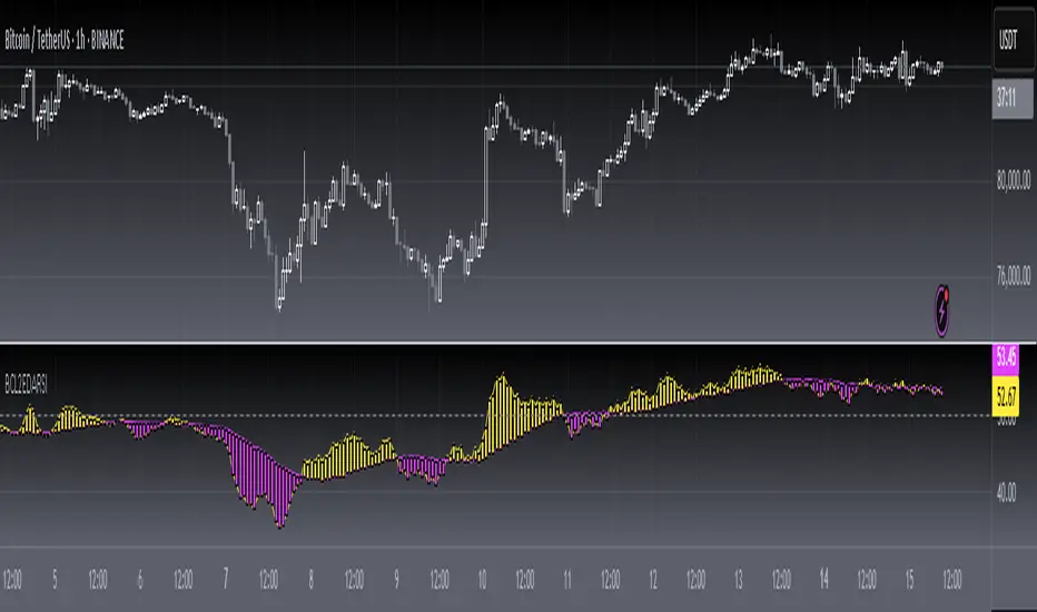
Discrete Fourier Transformed Money Flow IndexThe Discrete Fourier Transform Money Flow Index indicator integrates the Money Flow Index (MFI) with Discrete Fourier Transform (credit to author wbburgin - May 26 2023 ) smoothing to offer a refined and smoothed depiction of the MFI's underlying trend. The MFI is calculated using the formula: MFI = 100 - (100 / (1 + MR)), where a high MFI value indicates robust buying pressure (signaling an overbought condition), and a low MFI value indicates substantial selling pressure (signaling an oversold condition).
Why is the DFT and MFI combined?
The aim of this combination between DFT and MFI is to effectively filter out short-term fluctuations and noise, enabling a clearer assessment of the overall trend. This smoothing process enhances the reliability of the MFI by emphasizing dominant and sustained buying or selling pressures. This script executes a full DFT but only uses filtering from one frequency component. The choice to focus on the magnitude at index 0 is significant as it captures the dominant or fundamental frequency in the data. By analyzing this primary cyclic behavior, we can identify recurring patterns and potential turning points more easily. This streamlined approach simplifies interpretation and enhances efficiency by reducing complexity associated with multiple frequency components. Overall, focusing on the dominant frequency and applying it to the MFI provides a concise and actionable assessment of the underlying data.
Note: The FMFI indicator provides both smoothed and non-smoothed versions of the MFI, with the option to toggle the original non-smoothed MFI on or off in the settings.
Application
FMFI functions as a trend-following indicator. Bullish trends are denoted by the color white, while bearish trends are represented by the color purple. Circles plotted on the FMFI indicate regular bull and bear signals. Additionally, red arrows indicate a strong negative trend, while green arrows indicate a strong positive trend. These arrows are calculated based on the presence of regular bull and bear signals within overbought and oversold zones. To enhance its effectiveness, it is recommended to combine this indicator with other complementary technical analysis tools and integrate it into a comprehensive trading strategy. Traders are encouraged to explore a wide range of settings and timeframes to align the indicator with their unique trading preferences and adapt it to the current market conditions. By doing so, traders can optimize the indicator's performance and increase their potential for successful trading outcomes.
Utility
Traders and investors can employ this indicator to enhance their trend-following strategies. The white-colored components of the FMFI can help identify potential buying zones, while the purple-colored components can assist in identifying potential selling points. The red and green arrows can be used to pinpoint moments of strong bull or bear momentum, allowing traders to position themselves advantageously in their trading activities. Please note that future performance of any trading strategy is fundamentally unknowable, and past results do not guarantee future performance.

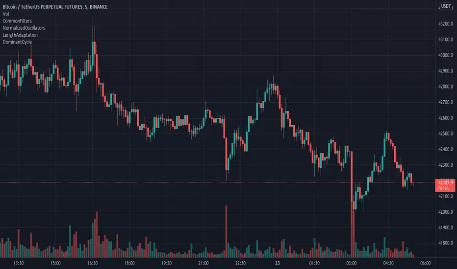
Adaptive Average Vortex Index [lastguru]As a longtime fan of ADX, looking at Vortex Indicator I often wondered, where is the third line. I have rarely seen that anybody is calculating it. So, here it is: Average Vortex Index - an ADX calculated from Vortex Indicator. I interpret it similarly to the ADX indicator: higher values show stronger trend. If you discover other interpretation or have suggestions, comments are welcome.
Both VI+ and VI- lines are also drawn. As I use adaptive length calculation in my other scripts (based on the libraries I've developed and published), I have also included the possibility to have an adaptive length here, so if you hate the idea of calculating ADX from VI, you can disable that line and just look at the adaptive Vortex Indicator.
Note that as with all my oscillators, all the lines here are renormalized to -1..1 range unlike the original Vortex Indicator computation. To do that for VI+ and VI- lines, I subtract 1 from their values. It does not change the shape or the amplitude of the lines.
Adaptation algorithms are roughly subdivided in two categories: classic Length Adaptations and Cycle Estimators (they are also implemented in separate libraries), all are selected in Adaptation dropdown. Length Adaptation used in the Adaptive Moving Averages and the Adaptive Oscillators try to follow price movements and accelerate/decelerate accordingly (usually quite rapidly with a huge range). Cycle Estimators, on the other hand, try to measure the cycle period of the current market, which does not reflect price movement or the rate of change (the rate of change may also differ depending on the cycle phase, but the cycle period itself usually changes slowly).
VIDYA - based on VIDYA algorithm. The period oscillates from the Lower Bound up (slow)
VIDYA-RS - based on Vitali Apirine's modification of VIDYA algorithm (he calls it Relative Strength Moving Average). The period oscillates from the Upper Bound down (fast)
Kaufman Efficiency Scaling - based on Efficiency Ratio calculation originally used in KAMA
Fractal Adaptation - based on FRAMA by John F. Ehlers
MESA MAMA Cycle - based on MESA Adaptive Moving Average by John F. Ehlers
Pearson Autocorrelation* - based on Pearson Autocorrelation Periodogram by John F. Ehlers
DFT Cycle* - based on Discrete Fourier Transform Spectrum estimator by John F. Ehlers
Phase Accumulation* - based on Dominant Cycle from Phase Accumulation by John F. Ehlers
Length Adaptation usually take two parameters: Bound From (lower bound) and To (upper bound). These are the limits for Adaptation values. Note that the Cycle Estimators marked with asterisks(*) are very computationally intensive, so the bounds should not be set much higher than 50, otherwise you may receive a timeout error (also, it does not seem to be a useful thing to do, but you may correct me if I'm wrong).
The Cycle Estimators marked with asterisks(*) also have 3 checkboxes: HP (Highpass Filter), SS (Super Smoother) and HW (Hann Window). These enable or disable their internal prefilters, which are recommended by their author - John F. Ehlers . I do not know, which combination works best, so you can experiment.
If no Adaptation is selected ( None option), you can set Length directly. If an Adaptation is selected, then Cycle multiplier can be set.
The oscillator also has the option to configure the internal smoothing function with Window setting. By default, RMA is used (like in ADX calculation). Fast Default option is using half the length for smoothing. Triangle , Hamming and Hann Window algorithms are some better smoothers suggested by John F. Ehlers.
After the oscillator a Moving Average can be applied. The following Moving Averages are included: SMA , RMA, EMA , HMA , VWMA , 2-pole Super Smoother, 3-pole Super Smoother, Filt11, Triangle Window, Hamming Window, Hann Window, Lowpass, DSSS.
Postfilter options are applied last:
Stochastic - Stochastic
Super Smooth Stochastic - Super Smooth Stochastic (part of MESA Stochastic ) by John F. Ehlers
Inverse Fisher Transform - Inverse Fisher Transform
Noise Elimination Technology - a simplified Kendall correlation algorithm "Noise Elimination Technology" by John F. Ehlers
Momentum - momentum (derivative)
Except for Inverse Fisher Transform , all Postfilter algorithms can have Length parameter. If it is not specified (set to 0), then the calculated Slow MA Length is used. If Filter/MA Length is less than 2 or Postfilter Length is less than 1, they are calculated as a multiplier of the calculated oscillator length.
More information on the algorithms is given in the code for the libraries used. I am also very grateful to other TradingView community members (they are also mentioned in the library code) without whom this script would not have been possible.

Adaptive MA Difference constructor [lastguru]A complimentary indicator to my Adaptive MA constructor. It calculates the difference between the two MA lines (inspired by the Moving Average Difference (MAD) indicator by John F. Ehlers). You can then further smooth the resulting curve. The parameters and options are explained here:
The difference is normalized by dividing the difference by twice its Root mean square (RMS) over Slow MA length. Inverse Fisher Transform is then used to force the -1..1 range.
Same Postfilter options are provided as in my Adaptive Oscillator constructor:
Stochastic - Stochastic
Super Smooth Stochastic - Super Smooth Stochastic (part of MESA Stochastic ) by John F. Ehlers
Inverse Fisher Transform - Inverse Fisher Transform
Noise Elimination Technology - a simplified Kendall correlation algorithm "Noise Elimination Technology" by John F. Ehlers
Momentum - momentum (derivative)
Except for Inverse Fisher Transform, all Postfilter algorithms can have Length parameter. If it is not specified (set to 0), then the calculated Slow MA Length is used.
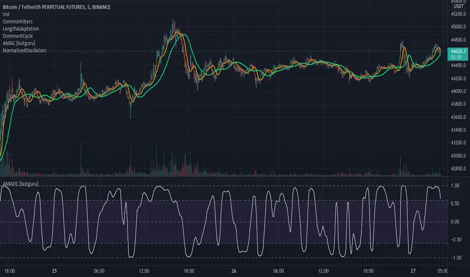
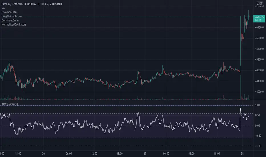
Adaptive Oscillator constructor [lastguru]Adaptive Oscillators use the same principle as Adaptive Moving Averages. This is an experiment to separate length generation from oscillators, offering multiple alternatives to be combined. Some of the combinations are widely known, some are not. Note that all Oscillators here are normalized to -1..1 range. This indicator is based on my previously published public libraries and also serve as a usage demonstration for them. I will try to expand the collection (suggestions are welcome), however it is not meant as an encyclopaedic resource , so you are encouraged to experiment yourself: by looking on the source code of this indicator, I am sure you will see how trivial it is to use the provided libraries and expand them with your own ideas and combinations. I give no recommendation on what settings to use, but if you find some useful setting, combination or application ideas (or bugs in my code), I would be happy to read about them in the comments section.
The indicator works in three stages: Prefiltering, Length Adaptation and Oscillators.
Prefiltering is a fast smoothing to get rid of high-frequency (2, 3 or 4 bar) noise.
Adaptation algorithms are roughly subdivided in two categories: classic Length Adaptations and Cycle Estimators (they are also implemented in separate libraries), all are selected in Adaptation dropdown. Length Adaptation used in the Adaptive Moving Averages and the Adaptive Oscillators try to follow price movements and accelerate/decelerate accordingly (usually quite rapidly with a huge range). Cycle Estimators, on the other hand, try to measure the cycle period of the current market, which does not reflect price movement or the rate of change (the rate of change may also differ depending on the cycle phase, but the cycle period itself usually changes slowly).
Chande (Price) - based on Chande's Dynamic Momentum Index (CDMI or DYMOI), which is dynamic RSI with this length
Chande (Volume) - a variant of Chande's algorithm, where volume is used instead of price
VIDYA - based on VIDYA algorithm. The period oscillates from the Lower Bound up (slow)
VIDYA-RS - based on Vitali Apirine's modification of VIDYA algorithm (he calls it Relative Strength Moving Average). The period oscillates from the Upper Bound down (fast)
Kaufman Efficiency Scaling - based on Efficiency Ratio calculation originally used in KAMA
Deviation Scaling - based on DSSS by John F. Ehlers
Median Average - based on Median Average Adaptive Filter by John F. Ehlers
Fractal Adaptation - based on FRAMA by John F. Ehlers
MESA MAMA Alpha - based on MESA Adaptive Moving Average by John F. Ehlers
MESA MAMA Cycle - based on MESA Adaptive Moving Average by John F. Ehlers , but unlike Alpha calculation, this adaptation estimates cycle period
Pearson Autocorrelation* - based on Pearson Autocorrelation Periodogram by John F. Ehlers
DFT Cycle* - based on Discrete Fourier Transform Spectrum estimator by John F. Ehlers
Phase Accumulation* - based on Dominant Cycle from Phase Accumulation by John F. Ehlers
Length Adaptation usually take two parameters: Bound From (lower bound) and To (upper bound). These are the limits for Adaptation values. Note that the Cycle Estimators marked with asterisks(*) are very computationally intensive, so the bounds should not be set much higher than 50, otherwise you may receive a timeout error (also, it does not seem to be a useful thing to do, but you may correct me if I'm wrong).
The Cycle Estimators marked with asterisks(*) also have 3 checkboxes: HP (Highpass Filter), SS (Super Smoother) and HW (Hann Window). These enable or disable their internal prefilters, which are recommended by their author - John F. Ehlers . I do not know, which combination works best, so you can experiment.
Chande's Adaptations also have 3 additional parameters: SD Length (lookback length of Standard deviation), Smooth (smoothing length of Standard deviation) and Power ( exponent of the length adaptation - lower is smaller variation). These are internal tweaks for the calculation.
Oscillators section offer you a choice of Oscillator algorithms:
Stochastic - Stochastic
Super Smooth Stochastic - Super Smooth Stochastic (part of MESA Stochastic) by John F. Ehlers
CMO - Chande Momentum Oscillator
RSI - Relative Strength Index
Volume-scaled RSI - my own version of RSI. It scales price movements by the proportion of RMS of volume
Momentum RSI - RSI of price momentum
Rocket RSI - inspired by RocketRSI by John F. Ehlers (not an exact implementation)
MFI - Money Flow Index
LRSI - Laguerre RSI by John F. Ehlers
LRSI with Fractal Energy - a combo oscillator that uses Fractal Energy to tune LRSI gamma
Fractal Energy - Fractal Energy or Choppiness Index by E. W. Dreiss
Efficiency ratio - based on Kaufman Adaptive Moving Average calculation
DMI - Directional Movement Index (only ADX is drawn)
Fast DMI - same as DMI, but without secondary smoothing
If no Adaptation is selected (None option), you can set Length directly. If an Adaptation is selected, then Cycle multiplier can be set.
Before an Oscillator, a High Pass filter may be executed to remove cyclic components longer than the provided Highpass Length (no High Pass filter, if Highpass Length = 0). Both before and after the Oscillator a Moving Average can be applied. The following Moving Averages are included: SMA, RMA, EMA, HMA , VWMA, 2-pole Super Smoother, 3-pole Super Smoother, Filt11, Triangle Window, Hamming Window, Hann Window, Lowpass, DSSS. For more details on these Moving Averages, you can check my other Adaptive Constructor indicator:
The Oscillator output may be renormalized and postprocessed with the following Normalization algorithms:
Stochastic - Stochastic
Super Smooth Stochastic - Super Smooth Stochastic (part of MESA Stochastic) by John F. Ehlers
Inverse Fisher Transform - Inverse Fisher Transform
Noise Elimination Technology - a simplified Kendall correlation algorithm "Noise Elimination Technology" by John F. Ehlers
Except for Inverse Fisher Transform, all Normalization algorithms can have Length parameter. If it is not specified (set to 0), then the calculated Oscillator length is used.
More information on the algorithms is given in the code for the libraries used. I am also very grateful to other TradingView community members (they are also mentioned in the library code) without whom this script would not have been possible.
Adaptive MA constructor [lastguru]Adaptive Moving Averages are nothing new, however most of them use EMA as their MA of choice once the preferred smoothing length is determined. I have decided to make an experiment and separate length generation from smoothing, offering multiple alternatives to be combined. Some of the combinations are widely known, some are not. This indicator is based on my previously published public libraries and also serve as a usage demonstration for them. I will try to expand the collection (suggestions are welcome), however it is not meant as an encyclopaedic resource, so you are encouraged to experiment yourself: by looking on the source code of this indicator, I am sure you will see how trivial it is to use the provided libraries and expand them with your own ideas and combinations. I give no recommendation on what settings to use, but if you find some useful setting, combination or application ideas (or bugs in my code), I would be happy to read about them in the comments section.
The indicator works in three stages: Prefiltering, Length Adaptation and Moving Averages.
Prefiltering is a fast smoothing to get rid of high-frequency (2, 3 or 4 bar) noise.
Adaptation algorithms are roughly subdivided in two categories: classic Length Adaptations and Cycle Estimators (they are also implemented in separate libraries), all are selected in Adaptation dropdown. Length Adaptation used in the Adaptive Moving Averages and the Adaptive Oscillators try to follow price movements and accelerate/decelerate accordingly (usually quite rapidly with a huge range). Cycle Estimators, on the other hand, try to measure the cycle period of the current market, which does not reflect price movement or the rate of change (the rate of change may also differ depending on the cycle phase, but the cycle period itself usually changes slowly).
Chande (Price) - based on Chande's Dynamic Momentum Index (CDMI or DYMOI), which is dynamic RSI with this length
Chande (Volume) - a variant of Chande's algorithm, where volume is used instead of price
VIDYA - based on VIDYA algorithm. The period oscillates from the Lower Bound up (slow)
VIDYA-RS - based on Vitali Apirine's modification of VIDYA algorithm (he calls it Relative Strength Moving Average). The period oscillates from the Upper Bound down (fast)
Kaufman Efficiency Scaling - based on Efficiency Ratio calculation originally used in KAMA
Deviation Scaling - based on DSSS by John F. Ehlers
Median Average - based on Median Average Adaptive Filter by John F. Ehlers
Fractal Adaptation - based on FRAMA by John F. Ehlers
MESA MAMA Alpha - based on MESA Adaptive Moving Average by John F. Ehlers
MESA MAMA Cycle - based on MESA Adaptive Moving Average by John F. Ehlers, but unlike Alpha calculation, this adaptation estimates cycle period
Pearson Autocorrelation* - based on Pearson Autocorrelation Periodogram by John F. Ehlers
DFT Cycle* - based on Discrete Fourier Transform Spectrum estimator by John F. Ehlers
Phase Accumulation* - based on Dominant Cycle from Phase Accumulation by John F. Ehlers
Length Adaptation usually take two parameters: Bound From (lower bound) and To (upper bound). These are the limits for Adaptation values. Note that the Cycle Estimators marked with asterisks(*) are very computationally intensive, so the bounds should not be set much higher than 50, otherwise you may receive a timeout error (also, it does not seem to be a useful thing to do, but you may correct me if I'm wrong).
The Cycle Estimators marked with asterisks(*) also have 3 checkboxes: HP (Highpass Filter), SS (Super Smoother) and HW (Hann Window). These enable or disable their internal prefilters, which are recommended by their author - John F. Ehlers. I do not know, which combination works best, so you can experiment.
Chande's Adaptations also have 3 additional parameters: SD Length (lookback length of Standard deviation), Smooth (smoothing length of Standard deviation) and Power (exponent of the length adaptation - lower is smaller variation). These are internal tweaks for the calculation.
Length Adaptaton section offer you a choice of Moving Average algorithms. Most of the Adaptations are originally used with EMA, so this is a good starting point for exploration.
SMA - Simple Moving Average
RMA - Running Moving Average
EMA - Exponential Moving Average
HMA - Hull Moving Average
VWMA - Volume Weighted Moving Average
2-pole Super Smoother - 2-pole Super Smoother by John F. Ehlers
3-pole Super Smoother - 3-pole Super Smoother by John F. Ehlers
Filt11 -a variant of 2-pole Super Smoother with error averaging for zero-lag response by John F. Ehlers
Triangle Window - Triangle Window Filter by John F. Ehlers
Hamming Window - Hamming Window Filter by John F. Ehlers
Hann Window - Hann Window Filter by John F. Ehlers
Lowpass - removes cyclic components shorter than length (Price - Highpass)
DSSS - Derivation Scaled Super Smoother by John F. Ehlers
There are two Moving Averages that are drown on the chart, so length for both needs to be selected. If no Adaptation is selected ( None option), you can set Fast Length and Slow Length directly. If an Adaptation is selected, then Cycle multiplier can be selected for Fast and Slow MA.
More information on the algorithms is given in the code for the libraries used. I am also very grateful to other TradingView community members (they are also mentioned in the library code) without whom this script would not have been possible.

DominantCycleCollection of Dominant Cycle estimators. Length adaptation used in the Adaptive Moving Averages and the Adaptive Oscillators try to follow price movements and accelerate/decelerate accordingly (usually quite rapidly with a huge range). Cycle estimators, on the other hand, try to measure the cycle period of the current market, which does not reflect price movement or the rate of change (the rate of change may also differ depending on the cycle phase, but the cycle period itself usually changes slowly). This collection may become encyclopaedic, so if you have any working cycle estimator, drop me a line in the comments below. Suggestions are welcome. Currently included estimators are based on the work of John F. Ehlers
mamaPeriod(src, dynLow, dynHigh) MESA Adaptation - MAMA Cycle
Parameters:
src : Series to use
dynLow : Lower bound for the dynamic length
dynHigh : Upper bound for the dynamic length
Returns: Calculated period
Based on MESA Adaptive Moving Average by John F. Ehlers
Performs Hilbert Transform Homodyne Discriminator cycle measurement
Unlike MAMA Alpha function (in LengthAdaptation library), this does not compute phase rate of change
Introduced in the September 2001 issue of Stocks and Commodities
Inspired by the @everget implementation:
Inspired by the @anoojpatel implementation:
paPeriod(src, dynLow, dynHigh, preHP, preSS, preHP) Pearson Autocorrelation
Parameters:
src : Series to use
dynLow : Lower bound for the dynamic length
dynHigh : Upper bound for the dynamic length
preHP : Use High Pass prefilter (default)
preSS : Use Super Smoother prefilter (default)
preHP : Use Hann Windowing prefilter
Returns: Calculated period
Based on Pearson Autocorrelation Periodogram by John F. Ehlers
Introduced in the September 2016 issue of Stocks and Commodities
Inspired by the @blackcat1402 implementation:
Inspired by the @rumpypumpydumpy implementation:
Corrected many errors, and made small speed optimizations, so this could be the best implementation to date (still slow, though, so may revisit in future)
High Pass and Super Smoother prefilters are used in the original implementation
dftPeriod(src, dynLow, dynHigh, preHP, preSS, preHP) Discrete Fourier Transform
Parameters:
src : Series to use
dynLow : Lower bound for the dynamic length
dynHigh : Upper bound for the dynamic length
preHP : Use High Pass prefilter (default)
preSS : Use Super Smoother prefilter (default)
preHP : Use Hann Windowing prefilter
Returns: Calculated period
Based on Spectrum from Discrete Fourier Transform by John F. Ehlers
Inspired by the @blackcat1402 implementation:
High Pass, Super Smoother and Hann Windowing prefilters are used in the original implementation
phasePeriod(src, dynLow, dynHigh, preHP, preSS, preHP) Phase Accumulation
Parameters:
src : Series to use
dynLow : Lower bound for the dynamic length
dynHigh : Upper bound for the dynamic length
preHP : Use High Pass prefilter (default)
preSS : Use Super Smoother prefilter (default)
preHP : Use Hamm Windowing prefilter
Returns: Calculated period
Based on Dominant Cycle from Phase Accumulation by John F. Ehlers
High Pass and Super Smoother prefilters are used in the original implementation
doAdapt(type, src, len, dynLow, dynHigh, chandeSDLen, chandeSmooth, chandePower, preHP, preSS, preHP) Execute a particular Length Adaptation or Dominant Cycle Estimator from the list
Parameters:
type : Length Adaptation or Dominant Cycle Estimator type to use
src : Series to use
len : Reference lookback length
dynLow : Lower bound for the dynamic length
dynHigh : Upper bound for the dynamic length
chandeSDLen : Lookback length of Standard deviation for Chande's Dynamic Length
chandeSmooth : Smoothing length of Standard deviation for Chande's Dynamic Length
chandePower : Exponent of the length adaptation for Chande's Dynamic Length (lower is smaller variation)
preHP : Use High Pass prefilter for the Estimators that support it (default)
preSS : Use Super Smoother prefilter for the Estimators that support it (default)
preHP : Use Hann Windowing prefilter for the Estimators that support it
Returns: Calculated period (float, not limited)
doEstimate(type, src, dynLow, dynHigh, preHP, preSS, preHP) Execute a particular Dominant Cycle Estimator from the list
Parameters:
type : Dominant Cycle Estimator type to use
src : Series to use
dynLow : Lower bound for the dynamic length
dynHigh : Upper bound for the dynamic length
preHP : Use High Pass prefilter for the Estimators that support it (default)
preSS : Use Super Smoother prefilter for the Estimators that support it (default)
preHP : Use Hann Windowing prefilter for the Estimators that support it
Returns: Calculated period (float, not limited)
JohnEhlersFourierTransformLibrary "JohnEhlersFourierTransform"
Fourier Transform for Traders By John Ehlers, slightly modified to allow to inspect other than the 8-50 frequency spectrum.
reference:
www.mesasoftware.com
high_pass_filter(source) Detrended version of the data by High Pass Filtering with a 40 Period cutoff
Parameters:
source : float, data source.
Returns: float.
transformed_dft(source, start_frequency, end_frequency) DFT by John Elhers.
Parameters:
source : float, data source.
start_frequency : int, lower bound of the frequency window, must be a positive number >= 0, window must be less than or 30.
end_frequency : int, upper bound of the frequency window, must be a positive number >= 0, window must be less than or 30.
Returns: tuple with float, float array.
db_to_rgb(db, transparency) converts the frequency decibels to rgb.
Parameters:
db : float, decibels value.
transparency : float, transparency value.
Returns: color.

MathSpecialFunctionsDiscreteFourierTransformLibrary "MathSpecialFunctionsDiscreteFourierTransform"
Method for Complex Discrete Fourier Transform (DFT).
dft(inputs, inverse) Complex Discrete Fourier Transform (DFT).
Parameters:
inputs : float array, pseudo complex array of paired values .
inverse : bool, invert the transformation.
Returns: float array, pseudo complex array of paired values .

[blackcat] L2 Ehlers DFT-Adapted RSILevel: 2
Background
John F. Ehlers introuced his DFT-ADAPTED RELATIVE STRENGTH INDEX (RSI) in Jan, 2007.
Function
In "Fourier Transform For Traders" in Jan, 2007, John Ehlers presented an interesting technique of improving the resolution of spectral analysis that could be used to effectively measure market cycles. Better resolution is obtained by a surprisingly simple modification of the discrete Fourier transform. John Ehlers suggests using the discrete Fourier transform (DFT) to tune indicators. Here, I demonstrate this by building a DFT-adapted relative strength index (RSI) strategy.
Rather than display the RSI for a single cycle length across the entire chart, Ehlers DFT adaptive RSI value reflects the DFT-calculated dominant cycle length RSI. If the dominant cycle changes from 14 to 18 bars, the RSI length parameter changes accordingly. Computationally, this requires the strategy to continuously update values for all possible RSI cycle lengths via a "for" loop and array.
In details, a full-featured formula that implements a high-pass filter (HP) and a six-tap low-pass finite impulse response (FIR) filter on input, then does discrete Fourier transform calculations. I has taken liberty of adding extra parameters so the user can modify the analysis window length and the high-pass filter cutoff frequency in real time using the parameters window. Once the suite of possible RSI values is calculated, we use the DFT to select the relevant RSI for the current bar. The strategy then trades according to J. Welles Wilder's original rules for the RSI.
Key Signal
fastline--> DFT-ADAPTED RELATIVE STRENGTH INDEX (RSI) fast line
slowline--> DFT-ADAPTED RELATIVE STRENGTH INDEX (RSI) slow line
Pros and Cons
100% John F. Ehlers definition translation, even variable names are the same. This help readers who would like to use pine to read his book.
Remarks
The 71th script for Blackcat1402 John F. Ehlers Week publication.
Based on original work of Ehlers, I added ALMA smoothing on DFT-adapted relative strength index (RSI) so that clearer trend can be observed.
Readme
In real life, I am a prolific inventor. I have successfully applied for more than 60 international and regional patents in the past 12 years. But in the past two years or so, I have tried to transfer my creativity to the development of trading strategies. Tradingview is the ideal platform for me. I am selecting and contributing some of the hundreds of scripts to publish in Tradingview community. Welcome everyone to interact with me to discuss these interesting pine scripts.
The scripts posted are categorized into 5 levels according to my efforts or manhours put into these works.
Level 1 : interesting script snippets or distinctive improvement from classic indicators or strategy. Level 1 scripts can usually appear in more complex indicators as a function module or element.
Level 2 : composite indicator/strategy. By selecting or combining several independent or dependent functions or sub indicators in proper way, the composite script exhibits a resonance phenomenon which can filter out noise or fake trading signal to enhance trading confidence level.
Level 3 : comprehensive indicator/strategy. They are simple trading systems based on my strategies. They are commonly containing several or all of entry signal, close signal, stop loss, take profit, re-entry, risk management, and position sizing techniques. Even some interesting fundamental and mass psychological aspects are incorporated.
Level 4 : script snippets or functions that do not disclose source code. Interesting element that can reveal market laws and work as raw material for indicators and strategies. If you find Level 1~2 scripts are helpful, Level 4 is a private version that took me far more efforts to develop.
Level 5 : indicator/strategy that do not disclose source code. private version of Level 3 script with my accumulated script processing skills or a large number of custom functions. I had a private function library built in past two years. Level 5 scripts use many of them to achieve private trading strategy.
[blackcat] L2 Ehlers DFT Spectral EstimateLevel: 2
Background
John F. Ehlers introduced DFT Spectral Estimate in his "Cycle Analytics for Traders" chapter 9 on 2013.
Function
The DFT is accomplished by correlating the data with the cosine and sine of each period of interest over the selected window period. The sum of the squares of each of these correlated values represents the relative power at each period. The only user input is whether to select Spectral Dilation compensation. The default selection is NOT to use the compensation.
The spectrum values vary between 0 and 1 after being normalized. These values are converted to colors. When the spectrum is greater than 0.5 the colors combine red and yellow, with yellow being the result when spectrum = 1 and red being the result when the spectrum = 0.5. When the spectrum is less than 0.5, the red saturation is decreased, with the result that the color is black when spectrum = 0.
Key Signal
DominantCycle --> Dominant Cycle signal
Pros and Cons
100% John F. Ehlers definition translation of original work, even variable names are the same. This help readers who would like to use pine to read his book. If you had read his works, then you will be quite familiar with my code style.
Remarks
The 51th script for Blackcat1402 John F. Ehlers Week publication.
Readme
In real life, I am a prolific inventor. I have successfully applied for more than 60 international and regional patents in the past 12 years. But in the past two years or so, I have tried to transfer my creativity to the development of trading strategies. Tradingview is the ideal platform for me. I am selecting and contributing some of the hundreds of scripts to publish in Tradingview community. Welcome everyone to interact with me to discuss these interesting pine scripts.
The scripts posted are categorized into 5 levels according to my efforts or manhours put into these works.
Level 1 : interesting script snippets or distinctive improvement from classic indicators or strategy. Level 1 scripts can usually appear in more complex indicators as a function module or element.
Level 2 : composite indicator/strategy. By selecting or combining several independent or dependent functions or sub indicators in proper way, the composite script exhibits a resonance phenomenon which can filter out noise or fake trading signal to enhance trading confidence level.
Level 3 : comprehensive indicator/strategy. They are simple trading systems based on my strategies. They are commonly containing several or all of entry signal, close signal, stop loss, take profit, re-entry, risk management, and position sizing techniques. Even some interesting fundamental and mass psychological aspects are incorporated.
Level 4 : script snippets or functions that do not disclose source code. Interesting element that can reveal market laws and work as raw material for indicators and strategies. If you find Level 1~2 scripts are helpful, Level 4 is a private version that took me far more efforts to develop.
Level 5 : indicator/strategy that do not disclose source code. private version of Level 3 script with my accumulated script processing skills or a large number of custom functions. I had a private function library built in past two years. Level 5 scripts use many of them to achieve private trading strategy.

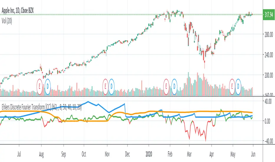
Ehlers Discrete Fourier TransformThe Discrete Fourier Transform Indicator was written by John Ehlers and more details can be found at www.mesasoftware.com
I have color coded everything as follows: blue line is the dominant cycle, orange line is the power converted to decibels, and I have marked the other line as red if you should sell or green if you should buy
Let me know if you would like to see me write any other scripts!
FUNCTION: Goertzel algorithm -- DFT of a specific frequency binThis function implements the Goertzel algorithm (for integer N).
The Goertzel algorithm is a technique in digital signal processing (DSP) for efficient evaluation of the individual terms of the discrete Fourier transform (DFT).
In short, it measure the power of a specific frequency like one bin of a DFT, over a rolling window (N) of samples.
Here you see an input signal that changes frequency and amplitude (from 7 bars to 17). I am running the indicator 3 times to show it measuring both frequencies and one in between (13). You can see it very accurately measures the signals present and their power, but is noisy in the transition. Changing the block len will cause it to be more responsive but noisier.
Here is a picture of the same signal, but with white noise added.
If you have a cycle you think is present you could use this to test it, but the function is designed for integration in to more complicated scripts. I think power is best interrupted on a log scale.
Given a period (in bars or samples) and a block_len (N in Goertzel terminology) the function returns the Real (InPhase) and Quadrature (Imaginary) components of your signal as well as calculating the power and the instantaneous angle (in radians).
I hope this proves useful to the DSP folks here.

Filter Amplitude Response Estimator - A Simple CalculationIn digital signal processing knowing how a system interact with the frequency content of an input signal is extremely important, the mathematical tool that give you this information is called "frequency response". The frequency response regroup two elements, the amplitude response, and the phase response. The amplitude response tells you how the system modify the amplitude of the frequency components in the input signal, the phase response tells you how the system modify the phase of the frequency components in the signal, each being a function of the frequency.
The today proposed tool aim to give a low resolution representation of the amplitude response of any filter.
What Is The Amplitude Response Of A Filter ?
Remember that filters allow to interact with the frequency content of a signal by amplifying, attenuating and/or removing certain frequency components in the input signal, the amplitude (also called magnitude) response of a filter let you know exactly how your filter change the amplitude of the frequency components in the input signal, another way to see the amplitude response is as a tool that tell you what is the peak amplitude of a filter using a sinusoid of a certain frequency as input signal.
For example if the amplitude response of a filter give you a value of 0.9 at frequency 0.5, it means that the filter peak amplitude using a sinusoid of frequency 0.5 is equal to 0.9.
There are several ways to calculate the frequency response of a filter, when our filter is a FIR filter (the filter impulse response is finite), the frequency response of the filter is the absolute value of the discrete Fourier transform (DFT) of the filter impulse response.
If you are curious about this process, know that the DFT of a N samples signal return N values, so if our FIR filter coefficients are composed of only 5 values we would get a frequency response of 5 values...which would not be useful, this is why we "pad" our coefficients with zeros, that is we add zeros to the start and end of our series of coefficients, this process is called "zero-padding", so if our series of coefficients is: (1,2,3,4,5), applying zero padding would give (0,0...1,2,3,4,5,...0,0) while keeping a certain symmetry. This is related to the concept of resolution, a low resolution amplitude response would be composed of a low number of values and would not be useful, this is why we use zero-padding to add more values thus increasing the resolution.
Making a Fourier transform in Pinescript is not doable, as you need the complex number i for computing a DFT, but thats not even the only problem, a DFT would not be that useful anyway (as the processes to make it useful in a trading context would be way too complex) . So how can we calculate a filter amplitude response without using a DFT ? The simple answer is by taking the peak amplitude of a filter using a sinusoid of a certain frequency as input, this is what the proposed tool do.
Using The Tool
The proposed tool give you a 50 point amplitude response from frequency 0.005 to 0.25 by default. the setting "Range Divisor" allow you to see the amplitude response by using a different range of frequency, for example if the range divisor is equal to 2 the filter amplitude response will be evaluated from frequency 0.0025 to 0.125.
In the script, filt hold the filter you want to see the frequency response, by default a simple moving average.
The position of the frequency response is defined by the "Show Amplitude Response At Bar Number" setting, if you want the frequency response to start at bar number 5000 then enter 5000, by default 10000. If you are not a premium set the number at 4000 and it should work.
amplitude response of a simple moving average of period 14, res = 2.
By default the amplitude response use an amplitude scale, a value of 1 represent an unchanged amplitude. You can use Dbfs (decibel full scale) instead by checking the "To Decibels (Full Scale)" setting.
Dbfs amplitude response, a value of 0 represent an unchanged amplitude.
Some Amplitude Responses
In order to prove the accuracy of the proposed tool we can compare the amplitude response given by the proposed tool with the mathematical function of the amplitude response of a simple moving average, that is:
abs(sin(pi*f*length)/(length*sin(pi*f)))
In cyan the amplitude response given by the proposed tool and in blue the above function. Below are the amplitude responses of some moving averages with period 14.
Amplitude response of an EMA, the EMA is a IIR filter, therefore the amplitude response can't be made by taking the DFT of the impulse response (as this ones has infinite length), however our tool can give its frequency response.
Amplitude response of the Hull MA, as you can see some frequencies are amplified, this is common with low-lag filters.
Gaussian moving average (ALMA), with offset = 0.5 and sigma = 6.
Simple moving average high-pass filter amplitude response
Center of gravity bandpass filter amplitude response
Center of gravity bandreject filter.
IMPORTANT!: The amplitude response of adaptive moving averages is not stationary and might change over time.
Conclusion
A tool giving the amplitude response of any filter has been presented, of course this method is not efficient at all and has a low resolution of 50 points (the common resolution is of 512 points) and is difficult to work with, but has the merit to work on Tradingview and can give the frequency response of IIR filters, if you really need to see the frequency response of a filter then i recommend you to use the function freqz from the scipy package.
I still hope you will enjoy using this tool to have a look at the amplitude responses of your favorite moving averages.
I'am aware of the current situation, however i'am somehow feeling left out from the pinescript community, let me know via PM if i have done something to you and i'll do my best to fix any problems i might have caused (or i might be being parano xD)

DFT - Dominant Cycle Period 8-50 bars - John EhlerThis is the translation of discret cosine tranform (DCT) usage by John Ehler for finding dominant cycle period (DC).
The price is first filtered to remove aliasing noise(bellow 8 bars) and trend informations(above 50 bars), then the power is computed.
The trick here is to use a normalisation against the maximum power in order to get a good frequency resolution.
Current limitation in tradingview does not allow to display all of the periods, still the DC period is plot after beeing computed based on the center of gravity algo.
The DC period can be used to tune all of the indicators based on the cycles of the markets. For instance one can use this (DC period)/2 as an input for RSI.
Hope you find this of some interrest.