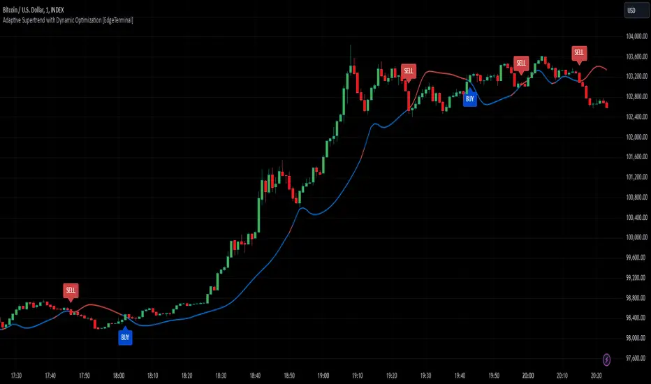
Adaptive Supertrend with Dynamic Optimization [EdgeTerminal]The Enhanced Adaptive Supertrend represents a significant evolution of the traditional Supertrend indicator, incorporating advanced mathematical optimization, dynamic volatility adjustment, intelligent signal filtering, reduced noise and false positives.
Key Features
Dynamic volatility-adjusted bands
Self-optimizing multiplier
Intelligent signal filtering system
Cooldown period to prevent signal clustering
Clear buy/sell signals with optimal positioning
Smooth trend visualization
RSI and MACD integration for confirmation
Performance-based optimization
Dynamic Band Calculation
Dynamic Band Calculation automatically adapts to market volatility, generates wider bands in volatile periods, reducing false signals. It also generates tighter bands in stable periods, capturing smaller moves and smooth transitions between different volatility regimes.
RSI Integration
The RSI and MACD play multiple crucial roles in the Adaptive Supertrend.
It first helps with momentum factor calculation. This dynamically adjusts band width based on momentum conditions. When the RSI is oversold, bands widen by 20% to prevent false signals during strong downtrends and provide more room for price movements in extreme conditions.
When the RSI is overbought, brands tighten by 20% and they become more sensitive to potential reversals to help catch trend changes earlier.
This reduces false signals in strong trends, helps detect potential reversals earlier than the usual, create adaptive band width based on market conditions and finally, better protection against whipsaws.
MACD Integration
The MACD in this supertrend indicator serves as a trend confirmation tool. The idea is to use MACD crossovers to confirm trend changes to reduce false trend change signals and enhance the signal quality.
For this to become a signal, MACD crossovers must align with price movement to help filter out weak or false signals, which acts as an additional layer of trend confirmation.
Additionally, MACD line position relative to signal line indicates trend strength, helps maintain positions in strong trends and assists in early detection of trend weakening.
Momentum Integration
Momentum Integration prevents false signals in extreme conditions, It adjusts dynamic bands based on market momentum, improves trend confirmation in strong moves and reduces whipsaws during consolidations.
Improved signals
There are a few systems to generate better signals, allowing for generally faster signals compared to original supertrend, such as:
Enforced cooldown period between signals
Prevents signal clustering
Clearer entry/exit points
Reduced false signals during choppy markets
Performance Optimization
This script implements a Sharpe ratio-inspired optimization algorithm to balance returns against risk, penalize large drawdowns, adapt parameters in real-time and improve risk-adjusted performance
Parameter Settings
ATR Period: 10 (default) - adjust based on timeframe
Initial Multiplier: 3.0 (default) - will self-optimize
Optimization Period: 50 (default) - longer periods for more stability
Smoothing Period: 3 (default) - adjust for signal smoothness
Best Practices
Use on multiple timeframes for confirmation
Allow the optimization process to run for at least 50 bars
Monitor the adaptive multiplier for trend strength indication
Consider RSI and MACD alignment for stronger signals
Dynamic
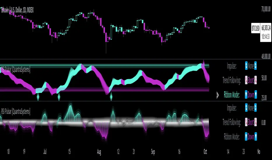
RSI Pulsar [QuantraSystems]RSI Pulsar
Introduction
The RSI Pulsar is an advanced and multifaceted tool designed to cater to the varying needs of traders, from long-term swing traders to higher-frequency day traders. This indicator takes the Relative Strength Index (RSI) to new heights by combining several unique methodologies to provide clear, actionable signals across different market conditions. With its ability to analyze impulsive trend strength, volatility, and binary market direction, the RSI Pulsar offers a holistic view of the market that assists traders in identifying robust signals and rotational opportunities within a volatile market.
The integration of dynamic color coding further aids in quick visual assessments, allowing traders to adapt swiftly to changing market conditions, making the RSI Pulsar an essential component in the arsenal of modern traders aiming for precision and adaptability in their trading endeavors.
Legend
The RSI Pulsar encapsulates various modes tailored to diverse trading strategies. The different modes are the:
Impulse Mode:
Focuses on strong outperformance, ideal for capturing movements in highly dynamic tokens.
Trend Following Mode:
A classical perpetual trend-following approach and provides binary long and short signal classifications ideal for medium term swing trading.
Ribbon Mode:
Offers quicker signals that are also binary in nature. Perfect for a confirmation signal when building higher frequency day trading systems.
Volatility Spectrum:
This feature projects a visual 'cloud' representing volatility, which helps traders spot emerging trends and potential breakouts or reversals.
Compressed Mode:
A condensed view that displays all signals in a clean and space-efficient manner. It provides a clear summary of market conditions, ideal for traders who prefer a simplified overview.
Methodology
The RSI Pulsar is built on a foundation of dynamic RSI analysis, where the traditional RSI is enhanced with advanced moving averages and standard deviation calculations. Each mode within the RSI Pulsar is designed to cater to specific aspects of the market's behavior, making it a versatile tool allowing traders to select different modes based on their trading style and market conditions.
Impulse Mode:
This mode identifies strong outperformance in assets, making it ideal for asset rotation systems. It uses a combination of RSI thresholds and dynamic moving averages to pinpoint when an asset is not just trending positively, but doing so with significant strength.
This is in contrast to typical usage of a base RSI, where elevated levels usually signal overbought and oversold periods. The RSI Pulsar flips this logic, where more extreme values are actually interpreted as a strong trend.
Trend Following Mode:
Here, the RSI is compared to the midline (the default is level 50, but a dynamic midline can also be set), to determine the prevailing trend. This mode simplifies the trend-following process, providing clear bullish or bearish signals based on whether the RSI is above or below the midline - whether a fixed or dynamic level.
Ribbon Mode:
This mode employs a series of calculated values derived from modified Heikin-Ashi smoothing to create a "ribbon" that smooths out price action and highlights underlying trends. The Ribbon Mode is particularly useful for traders who need quick confirmations of trend reversals or continuations.
Volatility Spectrum:
The Volatility Spectrum takes a unique approach to measuring market volatility by analyzing the size and direction of Heikin-Ashi candles. This data is used to create a volatility cloud that helps traders identify when volatility is rising, falling, or neutral - allowing them to adjust their strategies accordingly.
When the signal line breaks above the cloud, it signals increasing upwards volatility. When it breaks below it signifies increasing downwards volatility.
This can be used to help identify strengthening and weakening trends, as well as imminent volatile periods, allowing traders to position themselves and adapt their strategies accordingly. This mode also works as a great volatility filter for shorter term day trading strategies. It is incredibly sensitive to volatility divergences, and can give additional insights to larger market turning points.
Compressed Mode:
In Compressed Mode, all the signals from the various modes are displayed in a simplified format, making it easy for traders to quickly assess the market's overall condition without needing to delve into the details of each mode individually. Perfect for only viewing the exact data you need when live trading, or back testing.
Case Study I:
Utilizing ALMA Impulse Mode in High-Volatility Environments
Here, the RSI Pulsar is configured with an RSI length of 9 and an ALMA length of 2 in Impulse Mode. The chart example shows how this setup can identify significant price movements, allowing traders to enter positions early and capture substantial price moves. Despite the fast settings resulting in occasional false signals, the indicator's ability to catch and ride out major trends more than compensates, making it highly effective in volatile environments.
This configuration is suitable for traders seeking to trade quick, aggressive movements without enduring prolonged drawdowns. In Impulse Mode, the RSI Pulsar seeks strong trending zones, providing actionable signals that allow for timely entries and exits.
Case Study II:
SMMA Trend Following Mode for Ratio Analysis
The RSI Pulsar in Trend Following mode, configured with the SMMA with default length settings. This setup is ideal for analyzing longer-term trends, particularly useful in cryptocurrency pairs or ratio charts, where it’s crucial to identify robust directional moves. The chart showcases strong trends in the Solana/Ethereum pair. The RSI Pulsar’s ability to smooth out price action while remaining responsive to trend changes makes it an excellent tool for capturing extended price moves.
The image highlights how the RSI Pulsar efficiently tracks the strength of two tokens against each other, providing clear signals when one asset begins to outperform the other. Even in volatile markets, the SMMA ensures that the signals are reliable, filtering out noise and allowing traders to stay in the trend longer without being shaken out by minor corrections. This approach is particularly effective in ratio trading in order to inform a longer term swing trader of the strongest asset out of a customized pair.
Case Study III:
Monthly Analysis with RSI Pulsar in Ribbon Mode
This case study demonstrates the versatility and reliability of the RSI Pulsar in Ribbon mode, applied to a monthly chart of Bitcoin with an RSI length of 8 and a TEMA length of 14. This setup highlights the indicator’s robustness across multiple timeframes, extending even to long-term analysis. The RSI Pulsar effectively smooths out noise while capturing significant trends, as seen during Bitcoin bull markets. The Ribbon mode provides a clear visual representation of momentum shifts, making it easier for traders to identify trend continuations and reversals with confidence.
Case Study IV:
Divergences and Continuations with the Volatility Spectrum
Identifying harmony/divergences can be hit-or-miss at times, but this unique analysis method definitely has its merits at times. The RSI Pulsar, with its Volatility Spectrum feature, is used here to identify critical moments where price action either aligns with or diverges from the underlying volatility. As seen in the Bitcoin chart (using default settings), the indicator highlights areas where price trends either continue in harmony with volatility or diverge, signaling potential reversals. This method, while not always perfect, provides significant insight during key turning points in the market.
The Volatility Spectrum's visual representation of rising and falling volatility, combined with divergence and harmony analysis, enables traders to anticipate significant shifts in market dynamics. In this case, multiple divergences correctly identified early trend reversals, while periods of harmony indicated strong trend continuations. While this method requires careful interpretation, especially during complex market conditions, it offers valuable signals that can be pivotal in making informed trading decisions, especially if combined with other forms of analysis it can form a critical component of an investing system.
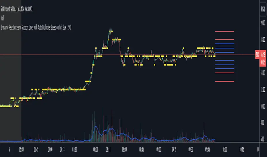
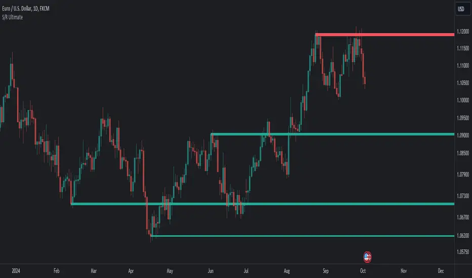
Dynamic Resistance and Support LinesThis script is designed to dynamically plot support and resistance lines based on full-dollar and half-dollar price levels relative to the close price on a chart. The script is particularly useful for day traders and scalpers, as it helps visualize key psychological price levels that often act as support and resistance zones in volatile and fast-moving markets in real time.
Key Features:
Dynamic Resistance and Support Levels:
Full-dollar levels: These are calculated by rounding the close price to the nearest full dollar and then extending the levels by adding and subtracting increments of 1 (e.g., $1, $2, $3).
Half-dollar levels: These are calculated by adding and subtracting 0.5 increments to the nearest full-dollar price, providing additional reference points. The historical full-dollar levels remain where support and resistance may have occurred in the past.
Extend Lines:
You can toggle whether the support and resistance lines are extended to the right, left, or both directions. This allows flexibility in projecting potential future areas of support or resistance.
Custom Line Extension:
The user can set the number of bars (or time periods) that the support and resistance lines will extend, giving control over how long the levels remain on the chart.
Color-Coded Lines:
Red lines represent full-dollar resistance and support levels.
Blue lines represent half-dollar levels, making it easy to differentiate between key psychological price zones.
Line Flexibility:
The script allows the lines to extend both left and right on the chart, making it useful for analyzing historical price action or projecting future price movements. The number of bars for extension is customizable, allowing for tailored setups.
Nearest Full Dollar Plot:
The nearest full-dollar price level is plotted as a yellow circle on the chart. This serves as a quick visual cue for traders to monitor price proximity to critical levels.
Benefits in Day Trading, Scalping, and Volatile Markets:
Visualizing Key Psychological Levels:
Full-dollar and half-dollar price levels often act as psychological barriers for traders. This script helps traders easily identify these levels, which are important in both fast-moving markets and during sideways consolidation.
Improved Decision-Making:
By automatically drawing these support and resistance levels, the script helps day traders and scalpers make quicker and more informed decisions, especially in volatile markets where every second counts.
Adaptability to Market Conditions:
The flexibility of extending lines based on trader preferences allows the user to adapt the script to various market conditions, such as high volatility or trend-based trading, providing a clear view of potential breakout or reversal areas.
Better Risk Management:
Having predefined support and resistance levels helps traders better manage risk, as these levels can act as logical areas for setting stop losses or taking profits.
This script is especially valuable for traders looking to capitalize on quick market movements or identify key entry and exit points during market volatility.
Dynamic Jurik RSX w/ Fisher Transform█ Introduction
The Dynamic Jurik RSX with Fisher Transform is a powerful and adaptive momentum indicator designed for traders who seek a non-laggy view of price movements. This script is based on the classic Jurik RSX (Relative Strength Index). It also includes features such as the dynamic overbought and oversold limits, the Inverse Fisher Transform, trend display, slope calculations, and the ability to color extremes for better clarity.
█ Key Features:
• RSX: The Relative Strength Index (RSX) in this script is based on Jurik’s RSX, which is smoother than the traditional RSI and aims to reduce noise and lag. This script calculates the RSX using an exponential smoothing technique and adaptive adjustments.
• Inverse Fisher Transform: This script can optionally apply the Inverse Fisher Transform to the RSX, which helps to normalize the RSX values, compressing them between -1 and 1. The inverse transformation makes it easier to spot extreme values (overbought and oversold conditions) by enhancing the visual clarity of those extremes. It also smooths the curve over a user-defined period in hopes of providing a more consistent signal.
• Dynamic Limits: The dynamic overbought and oversold limits are calculated based on the RSX's recent high and low values. The limits adjust dynamically depending on market conditions, making them more relevant to current price action.
• Slope Display: The slope of the RSX is calculated as the rate of change between the current and previous RSX value. The slope is displayed as dots when the slope exceeds the threshold designated by the user, providing visual cues for momentum shifts.
• Trend Coloring: Optionally, the user can also enable a trend-based display. It is simply based on current value of RSX versus the previous one. If RSX is rising then the trend is bullish, if not, then the trend is bearish.
• Coloring Extremes: Users can configure the RSX to color the chart when prices enter extreme conditions, such as overbought or oversold zones, providing visual cues for market reversals.
█ Attached Chart Notes:
• Top Panel: Enabled dynamic limits, Trend display, standard Jurik RSX with 20 lookback period, and Slope display.
• Middle Panel: Enabled dynamic limits, Extremes display, and standard Jurik RSX with 20 lookback period.
• Bottom Panel: Enabled dynamic limits, Trend display, Inverse Fisher Transform with 14 lookback period and 9 smoothing period. and Slope display.
█ Credits:
Special thanks to Everget for providing the original script. The script was also slightly modified based on updates from outside sources.
█ Disclaimer:
This script is for educational purposes only and should not be considered financial advice. Always conduct your own research and consult a professional before making any trading decisions.

Support Resistance UltimateThe "Support Resistance ULTIMATE" indicator is a comprehensive tool for traders on the TradingView platform, designed to identify key support and resistance levels using two primary techniques: pivot points and volume data. This indicator provides flexibility and customization, allowing traders to adapt it to their specific trading strategies.
KEY FEATURES
Pivot-Based Levels:
This feature calculates support and resistance levels using pivot points, which are derived from the high, low, and close prices of previous trading periods. Pivot points are crucial for forecasting potential market turning points.
Users can customize the pivot calculation by selecting the source type (either 'Close' or 'High/Low') and adjusting the lookback periods for both the left and right sides of the pivot calculation. This flexibility allows traders to adapt the indicator to different market conditions and timeframes.
Volume-Based Levels:
This option focuses on identifying support and resistance levels based on volume data, specifically the Point of Control (POC). The POC represents the price level with the highest traded volume during a specific time period, reflecting a consensus value among market participants.
The indicator includes a rolling POC calculation, allowing traders to dynamically assess areas of significant trading interest that may serve as support or resistance zones.
ADVANTAGES
Customization and Flexibility:
Traders can choose between pivot-based and volume-based levels or use both simultaneously, depending on their analysis needs. This dual approach provides a comprehensive view of market dynamics, accommodating various trading styles.
The indicator offers customizable color settings for support and resistance lines, enhancing chart readability and allowing traders to personalize their visual analysis.
Enhanced Market Insights:
By utilizing pivot points, traders can identify potential reversal or consolidation points, aiding in the prediction of market trends and the establishment of strategic entry and exit points.
Volume-based levels provide insights into market sentiment and participation, highlighting areas of strong support or resistance based on trading volume. This can improve risk management and trade execution by identifying high-probability trading zones.
Importance Scoring:
The indicator calculates the importance of each level based on the number of touches and the duration it holds. This scoring system helps traders assess the strength of support and resistance levels, with thicker lines indicating more significant levels.
This indicator is intended for educational and informational purposes only and should not be considered financial advice. Trading involves significant risk, and you should consult with a financial advisor before making any trading decisions. The performance of this indicator is not guaranteed, and past results do not predict future performance. Use at your own risk.
Three Anchored Moving Averages (VWAP / SMA / EMA)
This indicator allows users to anchor three types of moving averages (Simple Moving Average (SMA), Exponential Moving Average (EMA), and Volume Weighted Average Price (VWAP)) to specific points in time (anchor points)
Key Features:
Select from three Moving Average Types:
Simple Moving Average (SMA): Averages the closing prices over a specified period.
Exponential Moving Average (EMA): Gives more weight to recent prices, making it more responsive to new information.
Volume Weighted Average Price (VWAP): Averages the price weighted by volume, useful for understanding the average price at which the asset has traded over a period.
Up to Three Anchor Points:
Users can set up to three different anchor points to calculate the moving averages from specific dates and times. This allows for analysis of price action starting from significant points or specific events. For example, you can anchor to the low and high of a move to identify key levels or to points where the price takes off from a previous anchored MA.
Customisable Sentiment Options:
Each anchor point can be associated with a sentiment input (Auto, Bull, Bear, None), which influences if the MAs are displayed as lines or zones/bands:
Auto: Automatically determines the sentiment based on whether anchor points are on pivot highs and lows. If anchored to a pivot high, the system will assume a bearish sentiment and display a red band or zone between the MA OHLC4 and High. Anchoring to a pivot low will display a green band (OHLC4 - Low).
Bull: Forces a bullish sentiment (Green Band - OHLC4 to Low)
Bear: Forces a bearish sentiment (Red Band - OHLC4 to High)
None: Ignores sentiment and displays a single line (OHLC4)
Chart Matching:
The indicator includes an option to display the moving averages only if the chart symbol matches a specified ticker. This feature ensures that the indicator is relevant to the specific asset being analysed.
How to Use the Indicator:
1. Set Anchor Points: When added to your chart, select three anchor points by point and click. If you only wish to anchor to a single point, click on that point three times and disable the other two in settings once the indicator is applied.
2. Select Moving Average Type: Choose between SMA, EMA, or VWAP using the dropdown menu. EMAs are the most responsive.
3. Enable/Disable Anchor Points: Use the checkboxes to enable or disable each anchor point.
4. Select Sentiment Type: Choose between Auto, Bull, Bear, or None.
5. Chart Matching: Optionally, specify a chart symbol to restrict the indicator's display to that particular asset.
6. Interpret the Plots: The indicator plots the high, mid, and low values of the selected moving average type from each anchor point. The fills between these plots help identify potential support and resistance zones. These should be used as points of interest for pullback reversals or potential continuation if the price breaks through.
Practical Applications:
Trend Analysis: Identify the overall trend direction from specific historical points.
Support and Resistance: Determine key dynamic support and resistance levels based on anchored moving averages.
Event-Based Analysis: Anchor the moving averages to significant events (e.g., earnings releases, economic data) to study their impact on price trends.
Multi Timeframe Analysis: Higher Timeframe Anchors can be used to identify longer term trend analysis. Switching to a lower timeframe for execution triggers at these points wont distort the MA levels as they are anchored to a specific point in time
Intraday or Swing Trading: trend analysis using anchor points can be used for any style of trading (Intraday / Swing / Invest). Use anchored levels as points of interest and wait for hints in price action to try and catch the next move.

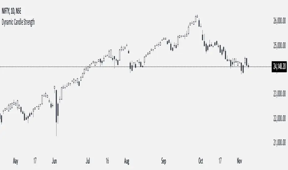
Dynamic Candle StrengthHow It Works
Initialization of Dynamic Levels:
The first candle's high and low are taken as the initial dynamic high and dynamic low levels.
If the next candle's close price is above the dynamic high, the candle is colored green, indicating bullish conditions.
If the next candle's close price is below the dynamic low, the candle is colored black, indicating bearish conditions.
If a candle's high and low crossed both the dynamic high and dynamic low, the dynamic high and low levels are updated to the high and low of that candle, but the candle color will continue with the same color as the previous candle.
Maintaining and Updating Dynamic Levels:
The dynamic high and low are only updated if a candle's close is above the current dynamic high or below the current dynamic low.
If the candle does not close above or below these levels, the dynamic high and low remain unchanged.
Visual Signals:
Green Bars: Indicate that the candle's close is above the dynamic high, suggesting bullish conditions.
Black Bars: Indicate that the candle's close is below the dynamic low, suggesting bearish conditions.
This method ensures that the dynamic high and low levels are adjusted in real-time based on the most recent significant price movements, providing a reliable measure of market sentiment.
Dynamic Order Blocks [LuxAlgo]The Dynamic Order Blocks indicator displays the most recent unmitigated bullish and bearish order blocks on the chart, providing dynamic support/resistance areas.
When price sweeps an order block, this is highlighted by the script indicating a potential reversal.
The average between the displayed order blocks is also displayed.
🔶 USAGE
Order blocks are a popular method of price action analysis, representing price areas where more significant market participants accumulate their orders.
Displaying order blocks dynamically allows obtaining relevant areas of support/resistance. Users can obtain longer-term order blocks using a higher "Swing Lookback" setting.
Users can also use mitigation events to assess the current trend direction, with price mitigating a bearish order block (breaking above the upper extremity) indicating an uptrend, and price mitigating a bullish order block (breaking below the lower extremity) indicating a downtrend.
🔹 Average Level
An average level obtained from the displayed bullish and bearish order blocks is included in the indicator and offers an additional polyvalent dynamic support/resistance level.
The change of direction of the average line can also be indicative of the current trend direction.
🔹 Dynamic Sweeps
Price sweeping the mitigation level of an order block is highlighted on the chart using bordered rectangles. These highlight a breakout failure and can be indicative of a potential reversal.
🔶 SETTINGS
Swing Lookback: Period of the swing detection used to construct order blocks. Higher values will return longer-term order blocks.
Use Candle Body: Use the candle body as the order block area instead of the candle full range.

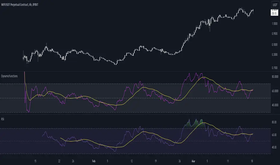
DynamicFunctionsLibrary "DynamicFunctions"
Custom Dynamic functions that allow an adaptive calculation beginning from the first bar
RoC(src, period)
Dynamic RoC
Parameters:
src (float) : and period
Custom function to calculate the actual period considering non-na source values
period (int)
dynamicMedian(src, length)
Dynamic Median
Parameters:
src (float) : and length
length (int)
kernelRegression(src, bandwidth, kernel_type)
Dynamic Kernel Regression Calculation Uses either of the following inputs for kernel_type: Epanechnikov Logistic Wave
Parameters:
src (float)
bandwidth (int)
kernel_type (string)
waveCalculation(source, bandwidth, width)
Use together with kernelRegression function to get chart applicable band
Parameters:
source (float)
bandwidth (int)
width (float)
Rsi(src, length)
Dynamic RSI function
Parameters:
src (float)
length (int)
dynamicStdev(src, period)
Dynamic SD function
Parameters:
src (float)
period (int)
stdv_bands(src, length, mult)
Dynamic SD Bands
Parameters:
src (float)
length (int)
mult (float)
Returns: Basis, Positive SD, Negative SD
Adx(dilen, adxlen)
Dynamic ADX
Parameters:
dilen (int)
adxlen (int)
Returns: adx
Atr(length)
Dynamic ATR
Parameters:
length (int)
Returns: ATR
Macd(source, fastLength, slowLength, signalSmoothing)
Dynamic MACD
Parameters:
source (float)
fastLength (int)
slowLength (int)
signalSmoothing (int)
Returns: macdLine, signalLine, histogram
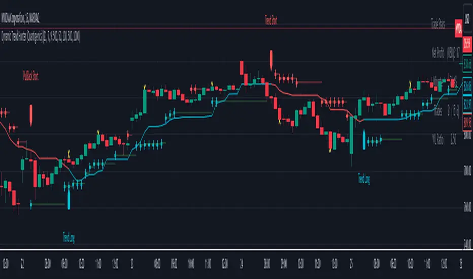
Dynamic Trend Hunter [Quantigenics]The "Dynamic Trend Hunter” script focuses on trend identification, dynamic entry and exit signals, and effective risk management. While a standalone trading script designed for versatile application across all markets, it can also be complemented by other indicators for enhanced analysis.
Core Features:
Dynamic Trend Indicator: Central to the script, this indicator discerns market trend direction using a color-coded system. Blue indicates an uptrend, red a downtrend, and a flat line signifies a sideways market.
Buy and Sell Signals: Provides clear, on-chart buy and sell signals to assist in identifying optimal entry points in alignment with the trend.
Profit Target Exits: A key feature designed to help traders lock in profits at strategic points. This feature uses a sophisticated mechanism (outlined in more detail below) to identify potential exit points, signaling the trader to close a position and secure gains before a potential market reversal.
Dynamic Stop Loss Levels: Essential for risk management, these levels adjust automatically, providing a mechanism for trailing stop losses and safeguarding against adverse market movements.
Technical Composition:
Dynamic Trend Indicator:
Calculation Method: Utilizes a blend of the highest and lowest prices over a specified length, averaged to create a trend line. This line is helpful in identifying the overall market trend.
Color Coding: The trend line changes color based on its relation to price action. A blue line indicates an uptrend when prices are consistently above this average line, while a red line signifies a downtrend when prices stay below it.
Signal-Based Trading:
Trend Entry Signals: Generated when there's a shift in the color of the trend line, indicating a potential change in market direction.
Pullback Entries: Identified when the closing price crosses the previous high (for long entries) or low (for short entries), while also considering the current trend line position.
Dynamic Stop Loss Levels:
Calculation: Stop loss levels are dynamically determined using the highest and lowest closing prices over the 'Length' period. These levels adjust with market movements, providing a trailing stop loss mechanism.
Visualization: Depicted as colored dots on the chart, changing in response to the market's movement relative to the trend line.
Oscillator for Dynamic Exits:
Mechanism: The script employs an oscillator to identify potential exit points, signaled by yellow dots. This oscillator is based on the relative extremity of the current price action compared to recent price movements.
Alerts: Dynamic exits trigger alerts when the oscillator reaches specified threshold levels, signaling potential market reversals or exhaustion points.
Customization and Flexibility:
Length Adjustment: The primary 'Length' input parameter allows traders to modify the sensitivity of the trend line and stop levels, catering to different trading styles and market conditions.
Alert Customization: Traders can set alerts for trend line changes and dynamic exits, ensuring timely responses to market movements.
Input Parameter Settings:
Intra-Bar Order Generation (IntraBar): Enables real-time signal generation within the current bar or after its closure.
Dynamic Exits (DynamicExits): Toggles the visibility of dynamic exit signals for profit-taking.
Dynamic Trend Length: Defines the lookback period for calculating the trend line. This length, which is adjustable and set by default to 21, specifies the number of bars over which the highest and lowest prices are analyzed to determine the trend line.
Dynamic Stop Loss Levels Length: This parameter defines the lookback period for calculating stop loss levels. It sets the number of bars used to determine the highest and lowest values for stop loss positioning. Adjusting this length allows traders to customize the sensitivity and placement of stop loss levels in accordance with their trading strategy and risk tolerance. This feature is crucial for tailoring stop loss settings to different market conditions and volatility levels, ensuring more effective risk management. Note: that initial stop loss levels, and tighter stop losses, can be set behind the Dynamic Trend Line itself.
Show Trend/Pullback Entries: Controls the display of specific entry signals based on trend continuation or market pullbacks.
Alert Settings: Options for setting alerts on trend line changes and dynamic exits, enhancing trade management.
Customizable Colors: Allows personalization of stop level and trend line colors for better chart visualization.
How to Trade with the Dynamic Trend Hunter:
Trend Following: Enter trades in the direction of the trend indicated by the color-coded trend line.
Pullback Entries: Look for pullback entry signals during established trends for additional entry points.
Dynamic Exits: Use yellow dot signals and dynamic stop loss levels for determining exit points or to adjust stop losses.
Risk Management: Employ the dynamic stop loss levels to manage risk effectively and protect against significant losses.
Alerts and Notifications:
Traders can set up alerts for trend line changes and dynamic exits, ensuring they are promptly informed about critical market movements and can react accordingly.
Conclusion:
The "Dynamic Trend Hunter " is a comprehensive and adaptable trading tool, suitable for various market conditions and trading styles. Its ability to provide clear trend indications, along with dynamic entry and exit signals, makes it an invaluable asset for traders aiming to enhance their market analysis and decision-making process. While it is a standalone system, it can be used in conjunction with other indicators to further refine trading strategies.
While we believe this tool may enhances your trading strategy, we encourage thorough familiarization before live trading. Remember, trading involves risk, and past performance is not indicative of future results.
You can see the “Author’s instructions" below to get immediate access to Dynamic Trend Hunter & the rest of the “Quantigenics Premium Indicator Suite”.
Advanced Dynamic Threshold RSI [Elysian_Mind]Advanced Dynamic Threshold RSI Indicator
Overview
The Advanced Dynamic Threshold RSI Indicator is a powerful tool designed for traders seeking a unique approach to RSI-based signals. This indicator combines traditional RSI analysis with dynamic threshold calculation and optional Bollinger Bands to generate weighted buy and sell signals.
Features
Dynamic Thresholds: The indicator calculates dynamic thresholds based on market volatility, providing more adaptive signal generation.
Performance Analysis: Users can evaluate recent price performance to further refine signals. The script calculates the percentage change over a specified lookback period.
Bollinger Bands Integration: Optional integration of Bollinger Bands for additional confirmation and visualization of potential overbought or oversold conditions.
Customizable Settings: Traders can easily customize key parameters, including RSI length, SMA length, lookback bars, threshold multiplier, and Bollinger Bands parameters.
Weighted Signals: The script introduces a unique weighting mechanism for signals, reducing false positives and improving overall reliability.
Underlying Calculations and Methods
1. Dynamic Threshold Calculation:
The heart of the Advanced Dynamic Threshold RSI Indicator lies in its ability to dynamically calculate thresholds based on multiple timeframes. Let's delve into the technical details:
RSI Calculation:
For each specified timeframe (1-hour, 4-hour, 1-day, 1-week), the Relative Strength Index (RSI) is calculated using the standard 14-period formula.
SMA of RSI:
The Simple Moving Average (SMA) is applied to each RSI, resulting in the smoothing of RSI values. This smoothed RSI becomes the basis for dynamic threshold calculations.
Dynamic Adjustment:
The dynamically adjusted threshold for each timeframe is computed by adding a constant value (5 in this case) to the respective SMA of RSI. This dynamic adjustment ensures that the threshold reflects changing market conditions.
2. Weighted Signal System:
To enhance the precision of buy and sell signals, the script introduces a weighted signal system. Here's how it works technically:
Signal Weighting:
The script assigns weights to buy and sell signals based on the crossover and crossunder events between RSI and the dynamically adjusted thresholds. If a crossover event occurs, the weight is set to 2; otherwise, it remains at 1.
Signal Combination:
The weighted buy and sell signals from different timeframes are combined using logical operations. A buy signal is generated if the product of weights from all timeframes is equal to 2, indicating alignment across timeframe.
3. Experimental Enhancements:
The Advanced Dynamic Threshold RSI Indicator incorporates experimental features for educational exploration. While not intended as proven strategies, these features aim to offer users a glimpse into unconventional analysis. Some of these features include Performance Calculation, Volatility Calculation, Dynamic Threshold Calculation Using Volatility, Bollinger Bands Module, Weighted Signal System Incorporating New Features.
3.1 Performance Calculation:
The script calculates the percentage change in the price over a specified lookback period (variable lookbackBars). This provides a measure of recent performance.
pctChange(src, length) =>
change = src - src
pctChange = (change / src ) * 100
recentPerformance1H = pctChange(close, lookbackBars)
recentPerformance4H = pctChange(request.security(syminfo.tickerid, "240", close), lookbackBars)
recentPerformance1D = pctChange(request.security(syminfo.tickerid, "1D", close), lookbackBars)
3.2 Volatility Calculation:
The script computes the standard deviation of the closing price to measure volatility.
volatility1H = ta.stdev(close, 20)
volatility4H = ta.stdev(request.security(syminfo.tickerid, "240", close), 20)
volatility1D = ta.stdev(request.security(syminfo.tickerid, "1D", close), 20)
3.3 Dynamic Threshold Calculation Using Volatility:
The dynamic thresholds for RSI are calculated by adding a multiplier of volatility to 50.
dynamicThreshold1H = 50 + thresholdMultiplier * volatility1H
dynamicThreshold4H = 50 + thresholdMultiplier * volatility4H
dynamicThreshold1D = 50 + thresholdMultiplier * volatility1D
3.4 Bollinger Bands Module:
An additional module for Bollinger Bands is introduced, providing an option to enable or disable it.
// Additional Module: Bollinger Bands
bbLength = input(20, title="Bollinger Bands Length")
bbMultiplier = input(2.0, title="Bollinger Bands Multiplier")
upperBand = ta.sma(close, bbLength) + bbMultiplier * ta.stdev(close, bbLength)
lowerBand = ta.sma(close, bbLength) - bbMultiplier * ta.stdev(close, bbLength)
3.5 Weighted Signal System Incorporating New Features:
Buy and sell signals are generated based on the dynamic threshold, recent performance, and Bollinger Bands.
weightedBuySignal = rsi1H > dynamicThreshold1H and rsi4H > dynamicThreshold4H and rsi1D > dynamicThreshold1D and crossOver1H
weightedSellSignal = rsi1H < dynamicThreshold1H and rsi4H < dynamicThreshold4H and rsi1D < dynamicThreshold1D and crossUnder1H
These features collectively aim to provide users with a more comprehensive view of market dynamics by incorporating recent performance and volatility considerations into the RSI analysis. Users can experiment with these features to explore their impact on signal accuracy and overall indicator performance.
Indicator Placement for Enhanced Visibility
Overview
The design choice to position the "Advanced Dynamic Threshold RSI" indicator both on the main chart and beneath it has been carefully considered to address specific challenges related to visibility and scaling, providing users with an improved analytical experience.
Challenges Faced
1. Differing Scaling of RSI Results:
RSI values for different timeframes (1-hour, 4-hour, and 1-day) often exhibit different scales, especially in markets like gold.
Attempting to display these RSIs on the same chart can lead to visibility issues, as the scaling differences may cause certain RSI lines to appear compressed or nearly invisible.
2. Candlestick Visibility vs. RSI Scaling:
Balancing the visibility of candlestick patterns with that of RSI values posed a unique challenge.
A single pane for both candlesticks and RSIs may compromise the clarity of either, particularly when dealing with assets that exhibit distinct volatility patterns.
Design Solution
Placing the buy/sell signals above/below the candles helps to maintain a clear association between the signals and price movements.
By allocating RSIs beneath the main chart, users can better distinguish and analyze the RSI values without interference from candlestick scaling.
Doubling the scaling of the 1-hour RSI (displayed in blue) addresses visibility concerns and ensures that it remains discernible even when compared to the other two RSIs: 4-hour RSI (orange) and 1-day RSI (green).
Bollinger Bands Module is optional, but is turned on as default. When the module is turned on, the users can see the upper Bollinger Band (green) and lower Bollinger Band (red) on the main chart to gain more insight into price actions of the candles.
User Flexibility
This dual-placement approach offers users the flexibility to choose their preferred visualization:
The main chart provides a comprehensive view of buy/sell signals in relation to candlestick patterns.
The area beneath the chart accommodates a detailed examination of RSI values, each in its own timeframe, without compromising visibility.
The chosen design optimizes visibility and usability, addressing the unique challenges posed by differing RSI scales and ensuring users can make informed decisions based on both price action and RSI dynamics.
Usage
Installation
To ensure you receive updates and enhancements seamlessly, follow these steps:
Open the TradingView platform.
Navigate to the "Indicators" tab in the top menu.
Click on "Community Scripts" and search for "Advanced Dynamic Threshold RSI Indicator."
Select the indicator from the search results and click on it to add to your chart.
This ensures that any future updates to the indicator can be easily applied, keeping you up-to-date with the latest features and improvements.
Review Code
Open TradingView and navigate to the Pine Editor.
Copy the provided script.
Paste the script into the Pine Editor.
Click "Add to Chart."
Configuration
The indicator offers several customizable settings:
RSI Length: Defines the length of the RSI calculation.
SMA Length: Sets the length of the SMA applied to the RSI.
Lookback Bars: Determines the number of bars used for recent performance analysis.
Threshold Multiplier: Adjusts the multiplier for dynamic threshold calculation.
Enable Bollinger Bands: Allows users to enable or disable Bollinger Bands integration.
Interpreting Signals
Buy Signal: Generated when RSI values are above dynamic thresholds and a crossover occurs.
Sell Signal: Generated when RSI values are below dynamic thresholds and a crossunder occurs.
Additional Information
The indicator plots scaled RSI lines for 1-hour, 4-hour, and 1-day timeframes.
Users can experiment with additional modules, such as machine-learning simulation, dynamic real-life improvements, or experimental signal filtering, depending on personal preferences.
Conclusion
The Advanced Dynamic Threshold RSI Indicator provides traders with a sophisticated tool for RSI-based analysis, offering a unique combination of dynamic thresholds, performance analysis, and optional Bollinger Bands integration. Traders can customize settings and experiment with additional modules to tailor the indicator to their trading strategy.
Disclaimer: Use of the Advanced Dynamic Threshold RSI Indicator
The Advanced Dynamic Threshold RSI Indicator is provided for educational and experimental purposes only. The indicator is not intended to be used as financial or investment advice. Trading and investing in financial markets involve risk, and past performance is not indicative of future results.
The creator of this indicator is not a financial advisor, and the use of this indicator does not guarantee profitability or specific trading outcomes. Users are encouraged to conduct their own research and analysis and, if necessary, consult with a qualified financial professional before making any investment decisions.
It is important to recognize that all trading involves risk, and users should only trade with capital that they can afford to lose. The Advanced Dynamic Threshold RSI Indicator is an experimental tool that may not be suitable for all individuals, and its effectiveness may vary under different market conditions.
By using this indicator, you acknowledge that you are doing so at your own risk and discretion. The creator of this indicator shall not be held responsible for any financial losses or damages incurred as a result of using the indicator.
Kind regards,
Ely

Dynamic Volume-Volatility Adjusted MomentumThis Indicator in a refinement of my earlier script PC*VC Moving average Old with easier to follow color codes, overbought and oversold zones. This script has converted the previous script into a standardized measure by converting it into Z-scores and also incorporated a volatility based dynamic length option. Below is a detailed Explanation.
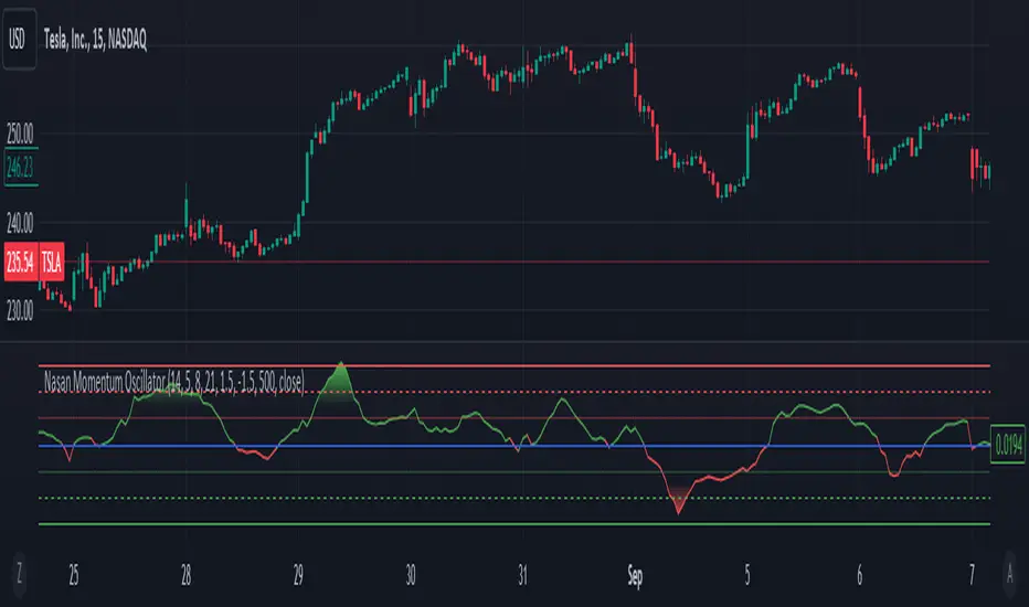
The "Dynamic Volume-Volatility Adjusted Momentum" or "Nasan Momentum Oscillator" is designed to capture market momentum while accounting for volume and volatility fluctuations. It leverages the Typical Price (TP), calculated as the average of high, low, and close prices, and introduces the Price Coefficient (PC) based on deviations from the simple moving average (SMA) across various time frames. Additionally, the Volume Coefficient (VC) compares current volume to SMA, and calculates Intraday Volatility (IDV) which gauges the daily price range relative to the close. Then intraday volatility ratio is calculated ( IDV Ratio) as the ratio of current Intraday Volatility (IDV) to the average of IDV for three different length periods, which provides a relative measure of current intraday volatility compared to its recent historical average. An inter-day ATR based Relative Volatility (RV) is calculated to adjusts for changing market volatility based on which the dynamic length adjustment adapts the moving average (standard length is 14). The PC *VC/IDV Ratio integrates price, volume, and volatility information which provides a volume and volatility adjusted momentum. This volume and volatility adjusted momentum is converted into a standardized Z-Score. The Z-Score measures deviations from the mean. Color-coded plots visually represent momentum, and thresholds aid in identifying overbought or oversold conditions.
The indicator incorporates a nuanced approach to emphasize the joint impact of price and volume while considering the stabilizing effect of lower intraday volatility. Placing the volume ratio (VC) in the numerator means that higher volume positively contributes to the overall ratio, aligning with the observation that increased volumes often accompany robust price movements. Simultaneously, the decision to include the inverse of intraday volatility (1/IDV) in the denominator acts as a dampener, reducing the impact of extreme intraday volatility on the momentum indicator. This design choice aims to filter out noise, giving more weight to significant price changes supported by substantial trading activity. In essence, the indicator's design seeks to provide a more robust momentum measure that balances the influence of price, volume, and volatility in the analysis of market dynamics.
TEWY - Magic Strength Indicator V2My goal is to equip every trader and investor with the essential tools necessary to confidently navigate the complexities of the financial markets, enabling them to consistently identify opportunities and maintain a position of strength on the winning side of their trades. This indicator stands as an immensely powerful tool, delivering a comprehensive and robust approach to market analysis and decision-making.
Allow me to provide some context regarding the genesis of this indicator. The global financial landscape encompasses a multitude of markets, ranging from the money market to the stock market, cryptocurrencies, commodities, and beyond. Often, these markets display proportional or inverse correlations, unveiling the intricate interplay between them. At the heart of this concept lies a meticulous comparison between a selected ticker and other analogous markets. This analytical approach serves as a pathway to unearthing invaluable insights and intricate patterns across interconnected sectors.
So, I created this indicator, to empower you with the capability to select and construct combinations of up to seven comparable markets and offer a comprehensive perspective on market dynamics.
Let me to elucidate the intricacies of this indicator and delve into its versatile configurations. By understanding its components and tailoring its settings, traders can harness its full potential to make informed and strategic trading decisions.
Related to indicator configuration sections
Section 1. 'PRIMARY AND SECONDARY INDEX' and Section 2. 'GLOBAL REFERENCE INDEX'
To utilize this indicator, begin by configuring at least one comparison indicator in the "Primary Index" field. Additional options include the secondary index (which can function as a sector index) and five global indices. Furthermore, you have the flexibility to adjust their timeframes, allowing for comparisons across various time horizons.
Section 3. ADVANCED FEATURS
Consider a scenario where you've pulled up a chart for "NSE:BANKNIFTY" and desire to assess the relative strength of "NSE:NIFTY" in comparison to global indices. To accomplish this, explore the Advanced Feature section and toggle the "Use Different Base Ticker" option to "Yes." Subsequently, input "NSE:NIFTY" as the symbol/ticker in the designated box. This ingenious feature empowers you to evaluate the strength of "NSE:NIFTY" the backdrop of the "NSE:BANKNIFTY" chart. The result? A remarkably potent analytical capability at your fingertips! The possibilities it offers are indeed remarkable!
Section 4. LINE AND BARCOLOR RELATED
I have dedicated considerable effort to scrutinize historical patterns within the strength indicator of various symbols. Through meticulous analysis, I've identified pivotal conditions that often herald shifts in market or symbol trends. Leveraging this insight, I've devised a system to determine optimal strength line colors and bar colors. This strategic approach adds a layer of precision to the indicator, enhancing its effectiveness in recognizing and visualizing trend changes.
Recognizing the prevailing tendency of global markets to exhibit more upward momentum than downward movement, I've taken into account this inherent "Long Bias." With this understanding in mind, I've incorporated a unique feature that aims to prompt an early transition from red to green bar colors when there's a potential indication of a trend reversal from a downtrend. By proactively signaling the shift in color dynamics, this feature aligns with the overall upward-leaning nature of the markets, enabling traders/investors to respond swiftly to potential changes in trend direction.
By employing the 'Use Simple Method of Calculation,' the determination of strength line color is executed through a straightforward crossover technique. This approach proves particularly effective in scenarios where inverse correlations exist between the symbols or tickers being compared. Additionally, an 'Inverse Scale' option is available, wherein a simple multiplication by -1 is applied to all values. This ingenious feature offers a convenient perspective on symbols or tickers that exhibit inverse correlations, further enhancing the indicator's adaptability to a wide array of market dynamics.
**** It's important to note that the 'Change Bar Color' option is intentionally set to the default selection of 'No.' By design, only when you opt to set it to 'Yes' do custom bar colors come into play on the chart. This thoughtful design choice acknowledges the potential need to preserve bar colors when seeking to discern inverse correlations between symbols. Should you require a modification in bar colors, kindly select 'Yes' to initiate this change and access the custom color functionality.
Section 5. LABELS
Moreover, to facilitate ease of use and organization, I've included a practical feature for instances where you deploy this indicator multiple times on a single chart. Within this context, should you wish to assign quick tags to each instance, a dedicated free-text box is at your disposal. This allows you to conveniently label and categorize different instances of the indicator, ensuring a streamlined and efficient approach to managing your chart analyses.
I encourage you all to embark on a rewarding journey in your trading and investing endeavors. With this indicator as your ally, equipped with its potent analytical capabilities, may your path be marked by well-informed decisions and prosperous outcomes. Wishing you every success in your trading and investment journey!
Should you have any inquiries or require further clarification regarding this indicator, please do not hesitate to reach out to me via direct message. I am here to provide you with the necessary guidance and support to ensure your experience with this tool is both seamless and enriching. Your understanding and satisfaction remain my utmost priority.
By TEWY - Trade Easy With Yogesh
I am Yogesh

KeitoFX Dynamic Indicator Free vers.This script represents a versatile dynamic indicator called "KeitoFX Dynamic Indicator Free version." It is developed by the author "KeitoFX" and operates as a custom indicator overlaying on financial charts. The indicator utilizes a unique algorithm to dynamically identify bullish and bearish candlestick patterns with specific criteria.
Key Features:
- The indicator visually marks bullish and bearish candlestick patterns using triangle shapes, providing quick visual cues to traders.
- Bullish patterns are detected when the closing price is higher than the opening price and the high and low prices of the candlestick form a narrow range.
- Bearish patterns are identified when the closing price is lower than the opening price, and the high and low prices also form a narrow range.
The indicator incorporates flexible settings that users can customize to fit their trading preferences:
- Users can choose the table's placement, either at the "Top Right," "Middle Right," or "Bottom Right" of the chart.
- Customizable dimensions for the width and height of the table are available.
- Adjustable text size settings ranging from "Auto" to "Huge" are provided for the displayed text.
- A descriptive table containing trading rules and conditions is optionally displayed below the price chart.
Additional Information:
- The indicator's color scheme is harmonious, with shades of purple and neutral tones.
- The "Require FVG" setting influences the pattern detection's sensitivity.
- A dynamic standard deviation is calculated based on the selected displacement settings and historical candle ranges.
- A "FVG" condition enhances pattern accuracy.
- Bullish and bearish pattern detection includes overlapping with other predefined arrays to increase pattern significance.
Note:
This indicator is provided under the Mozilla Public License 2.0, as indicated by the source code comment at the beginning of the script. Users are encouraged to review and comply with the license terms when using this indicator in their trading activities.

Dynamic Stop Loss DemoWhat does this script do ?
This script is for pine script programmers and explains how to implement a dynamic stop-loss strategy. It is different from trailing stop-loss. Trailing stop-loss can only set the retracement value, but this script can take profit on part of the position at a fixed price and allows users to decide whether to take profit on all positions based on whether a certain track is breached or other conditions author want. In this demo, it use rsi crossover and crossunder to decide the strategy condition, and use close price as open price, and use lowest low / highest high as stop price, and use 1.5 risk ratio to calculate the fixed first profit price. It will take 50% position size when the first profit price was reached. Then it will close all rest positions when the inverse condition come out or the dynamic stop(calculated by ATR) breached or when the price back to the open price or the stop price.
How is this script implemented
When start strategy by strategy.entry , it gives a custom id which contains direction, openPrice, stopPrice, profitPrice, qty, etc. It can be get from the global variable strategy.posiition_entry_name .

Anchored Moving Averages - InteractiveWhat is an Anchored Moving Average?
An anchored moving average (AMA) is created when you select a point on the chart and start calculating the moving average from there.
Thus the moving average’s denominator is not fixed but cumulative and dynamic. It is similar to an Anchored VWAP, but neglecting the volume data, which may be useful when this data is not reliable and you want to focus just on price.
Main Features
This interactive indicator allows you to select 3 different points in time to plot their respective moving averages. As soon as you add the indicator to your chart you will be asked to click on the 3 different points where you want to start the calculation for each moving average.
Each AMA (Anchored Moving Average) will be colored according to its slope, using a gradient defined by two user chosen colors in the indicator menu.
The default source for the calculation is the pivot price (HLC3) but can also be modified in the menu.
Examples:
Enjoy!
NDOG & Dynamic Event Horizon° (Experimental)The ICT concept of New Day Opening Gaps (NDOG) is simply an imbalance that may manifest at Daily Opening time. This gap in price is formed by the Close at 5PM EST and the open at 6PM EST.
According to ICT's studies, this gap in price holds a lot of significance when it comes to price action, acting as a magnet or a point of reference during the day (and following days/weeks).
This script applies the supporting concepts of New Week Opening Gaps (Event Horizon and OTE areas) to NDOGs, mimicking my NWOG & Dynamic Event Horizon° indicator. Equally to the latter, this script dynamically selects the most relevant NDOG Dealing Range and plots their EH and OTE levels automatically.
// Please refer to the NWOG indicator post linked above for more information about these concepts
Available Alerts:
– Cross Below Event Horizon
– Cross Above Event Horizon
– New NDOG Range Established
Important Remarks:
– This is purely an experiment, and has not been taught by ICT publicly in any way. Treat this material accordingly.
– Note that although these work on all timeframes, the lower in resolution one goes, the less gaps will be available due to data availability.
– This indicator works on charts that have the NDOG already present in chart (i.e. no crypto assets, unless one looks at CME crypto futures such as BTC1! and ETH1! ).
– The dollar index's NDOGs have a slightly different timestamp, however this has been taken care of and will allow to be plotted ONLY for the TVC:DXY ticker.
TrandingView struggles to display the indicator correctly for the default view, check out its accurate appearance here:

Waddah Attar Explosion with TDI First of all, a big shoutout to @shayankm, @LazyBear, @Bromley, @Goldminds and @LuxAlgo, the ones that made this script possible.
This is a version of Waddah Attar Explosion with Traders Dynamic Index.
WAE provides volume and volatility information. Also, WAE calculation was changed to a full-on MACD, to provide the momentum: the idea is to "assess" which MACD bars have significant momentum (i.e. crossover the Explosion Line)
TDI provides momentum, divergences as well as overbought and oversold areas. There is also a RSI on a different timeframe, for convergence.
Almost everything is editable:
- All moving averages are customizable, including the TRAMA, from @LuxAlgo
Waddah Attar Explosion_
- Three different crossing signals: histogram crossing contracting Explosion Line, expanding Explosion Line and ascending Explosion Line while both Bolling Bands are expanding; Explosion Line shows different color when expanding.
- Explosion line signals: Below DeadZone line and Exhaustion (highest value in a given lookback period). You can set a predefined EPL slope to filter out some noise.
- Deadzone signal : Deadzone squeeze ( lowst value in a given lookback period)
TDI:
- Overbought an Oversold signals. The OB and OS shapes have two colors, in order to display extreme signals on current timeframe or extreme signals on current and different time frame.
- Visual display of RSI outside the Bollinger Bands, and crossing of RSI Moving Average crossing of zero line.
I believe this combination is great for so many reasons!
Like the idea of TTM Squeeze? You can tune the Deadzone and Explosion lines to look for a volatility breakout
Like trading divergences or want to filter out extreme areas? The RSI is great for that
You like the using the MACD strategy but don't like the amount of false signals given? this WAE version filters some of them out.
If you are a Bollinger bands fan, you can customize both indicators to trade breakouts and/or mean reversion strategies, and filter out exhaustion of the bands expansion
This is my first publication, so give it a go and provide feedback if possible.
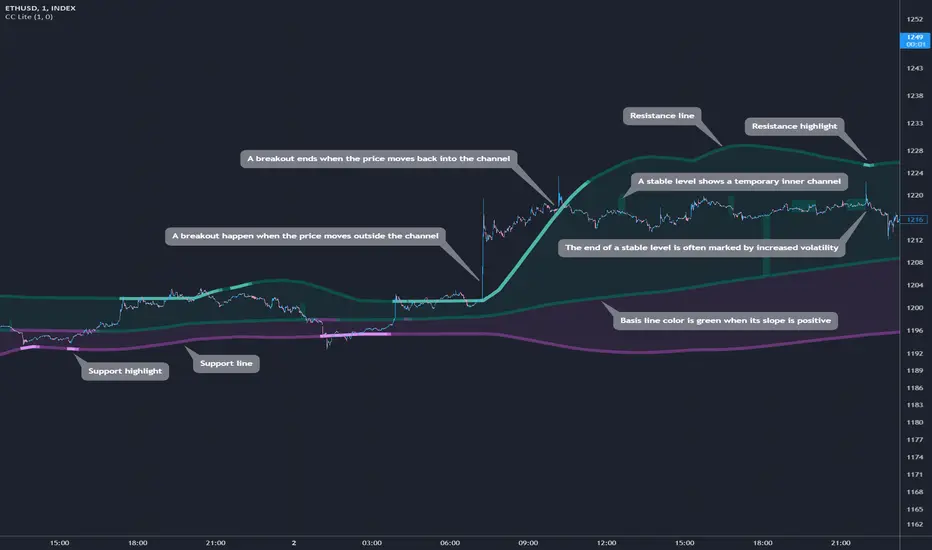
Cosmic Channel LiteCosmic Channel Lite ( CC Lite) draws dynamic non-repainting trendlines and helps
⭐ know when a breakout is about to begin
⭐ predict the position and timing of the next swing reversal
⭐ predict sudden changes in volatility
⭐ recognize whether the price is in bearish or bullish territory
👀 HOW IT WORKS
Cosmic Channel Lite draws a dynamic channel consisting of a support line, basis line and resistance line. These are calculated by applying the Reduced Median Method to groups of moving averages of different type over several periods each, effectively taking 20 data points and reducing them to 3. In between, 6 internal levels are left to give context inside the channel with stable levels, the extremes of which help highlight the SR lines (see chart). The basis line color is determined by its smoothed angle with positive angles in green and negative in purple. The aim of this indicator is to provide a consistent and generic price context that works out-of-the-box and accordingly the settings have been stripped to the bare minimum with no need to continually adjust them.
📗 HOW TO USE IT
The Cosmic Channel Lite plots are meant to be used as a guide for entering and exiting positions and setting stop-loss and take profit levels. The indicator is deemed effective for any particular timeframe as long as the price stays within the maximum bounds of the indicator's plots. For this reason it is recommended to use Cosmic Channel Lite in a multi-chart layout where each chart has a different timeframe. The 5 primary strategies are:
long when the price reverses off of the support line and short when the price reverses off of the resistance line
long when the support line is highlighted and short when the resistance line is highlighted
long when the price breaks above the resistance line and short when the price breaks below the support line
long when the price moves above the basis line after being below it for a prolonged period and visa-versa (short when the price moves below the basis line)
long/short in the direction the price takes after a stable level ends
🔔 SMART ALERTS
Get notified at the most critical times by settings just one alert. Simply select CC Lite and Any alert() function call as the conditions when creating an alert and you will be tipped-off on bar-close as follows:
R─ (resistance line is highlighted)
S─ (support line is highlighted)
For example, an alert such as CC Lite 6h R─ would mean that during the last 6-hour bar the resistance line has been highlighted. The highlight lasts at least 15 bars from the first highlight bar regardless of price action.
Entry helperHello traders,
This is a script I use daily as a scalper and it helps me a lot, maybe it can help you, this is why I am sharing it!
PART 1 - DESCRIPTION
This program is specifically designed to help scalpers but can be used for all types of trading but won't be as useful.
This script is what I call an entry helper as it calculates dynamically the position size, stop loss and take profit levels and more.
When scalping and placing market entry orders, the price can move significantely while you are calculating your position size according to your stop loss, capital, risk and especially close price that changes very quickly, this results in a risk that is not ideally controlled and personally was a source of frustration and stress. I wanted to enter my quantity and stop loss values as fast as possible and make the process easier.
This script automates the calculation of the position size, stop loss and take profit levels according the the users input and prints the data visibly on the screen so it is easy to copy by the trader. It allows the trader to be confident that his risk is as controlled as possible.
The script is easy to use and set up, this guide will help you if you have any difficulies or questions.
PART 2 - HOW TO USE THE SCRIPT
- SET THE CAPITAL SETTINGS
1 - Set your capital value in $
- SET THE TRADE SETTINGS
2 - Set your trade side (BUY or SELL)
3 - Set you desired risk in % of your capital
- ENTRY SETTINGS
4 - Set your entry from 2 different options
|MARKET| (default option)
This option will place the entry level at the last available price
|LIMIT|
This option allows you to input a fixed price level for the entry
- STOP LOSS SETTINGS
5 - Select your stop loss placement from 4 different options
|EXTREMA STOP LOSS| (default option)
This option will place the stop loss at the highest/lowest (extrema) price level within the last N candles
|ATR EXTREMA|
This option uses the same price level as the EXTREMA STOP LOSS but will add/soustract the last ATR value (calculated on the N last candles) multiplied by a coefficient that you input
|TICKS EXTREMA|
This option uses the same price level as the EXTREMA STOP LOSS but will add/soustract a number of ticks that you input
|PRICE LEVEL|
This option allows you to input a fixed price level for the stop loss
- TAKE PROFIT SETTINGS
6 - Select your take profit from 3 different options
|NONE| (default option)
This option will not display any take profit level, I have added this option as I don't have take profit targets
|RR|
This option uses a risk to reward ratio (reward/risk) that you input, it will automatically calculate the take profit level that corresponds
|PRICE LEVEL|
This option allows you to input a fixed price level for the take profit
- QUANTITY AND FEE SETTINGS
7 - Set the quantity settings, it represents the quantity in a lot (usually 100 000 in forex, 100 in stocks 1 for crypto currencies)
8 - Set the fee per quantity (turning lot)
- VISUAL SETTINGS
9 - Show or remove the tab
- TAB SETTINGS
10 - Select the data that you want to display in the tab (the tab will adapt automatically)
NOTES:
The vertical dashed line shows what candle has been used for the calculation of the stop loss, it allows you to visualize what candle the script has selected in case of an EXTREMA stop loss option.
I hope this helps you out! Any suggestions are welcome and I hope that the guide is clear enough.
Happy trading!

Dynamic Highest Lowest Moving AverageSimilar to my last script, although this one uses the RSI value of
(highest high - price) / (price - lowest low)
to feed into the the logic creating the dynamic length. Choose how the length curve works by selecting either Incline, Decline, Peak or Trough.
Lastly select the moving average type to filter the result through to smoothen things out a bit
to find something that works for your strategy. This is useful as an entry/exit indicator along with other moving averages, or even just a standalone if you play with the settings enough.
TwV Multi-timeframe Dynamic VRVPMulti-timeframe Dynamic Visible Range Volume Profile
The volume profile is an indicator that displays trading activity over a specified period and plots a histogram on the chart which reveals dominant and significant price levels based on volume and in essence gives a clear indication of Supply or demand at a certain price rather than volume in a certain period.
What makes this VRVP indicator different from other is that it is multi-timeframe and dynamic, meaning that it has the ability to show the POC for a higher timeframe and that it also recalculates the main POC every single time traders adjust the chart.
Most VRVP need to be adjusted to a fixed position for the Main POC, I made an improvement by giving the indicator the ability to identify the bars that are being look at in the screen, this really gives traders the possibility and agility to identify potential support and resistance areas without the need to be changing any settings on the indicator.
Furthermore, giving the ability to the indicator to be multi-timeframe allows traders not only to work with a point of control in one timeframe, but also have a dashed line plotting the Point of Control of a HIGHER timeframe, which could potentially be a strongest support or resistance. The multi-timeframe point of control is fixed only.
This VRVP is completely similar to the official Trading View paid subscription one.
Fundamentals
Point of Control (POC): The price level for the time period with the highest traded volume. The POC is represented by an amber line within the indicator.
Profile High: The highest reached price level during the specified time period
Profile Low: The lowest reached price level during the specified time period.
Value Area (VA): The range of price levels in which a specified percentage of all volume was traded during the time period. Typically, this percentage is set to 70% however it is up to the trader’s discretion.
Value Area High (VAH): The highest price level within the value area.
Value Area Low (VAL): The lowest price level within the value area.
Usage
The Resistance and Support levels can be provided by the Volume profile using a reactive method so they constantly change with price action and give a clearer picture to predict future price movements. The Reactive method relies on past price movements at certain price levels and applies a more significant understanding of price reaction at certain meaningful levels
Support levels will be areas where price will be supported on the way down.
Resistance levels will be areas that resist price on the way up.
A basic understanding of this is that Buyers will enter the market at the bottom of a profile and sellers will enter the market at the top of the profile.
Configuration
By the default the indicator has enabled plotting the charts timeframe Volume Profile.
Multi-timeframe option needs to be enabled and desired timeframe chosen from selector menu.
Bars back value for fixed calculation of the multi-timeframe point of control.
Traders can adjust default settings as follows:
Charts timeframe VRVP
Main POC color – Yellow
Positive Volume – Green
Negative Volume – Red
VRVP Width – 100 (Refers to the plotting width for better suiting on small screens)
Multi timeframe VRVP
Enable or disable calculations
Bars back - Fixed numbers of bars for calculation (Consider that max bars back limit is 5000, but it considers 5000 bars on the current charts timeframe, therefore traders need to take into consideration converting number of bars in higher timeframe to charts timeframe)
e.g.
Charts timeframe 15m – MTF desired 1H
1H = 60 min 15m = 15 min – 100 bars back equivalent to (60 min * 100) / 15 = 400
Lower than 5000 then calculations takes place, otherwise calculations will be disabled.
Multi-timeframe POC color = Light blue DASHED
Timeframe desired – 1H by default
Summary box
Enable or disable box
Box shows information regarding the exact price where Main POC and MTF POC reside
Table Size for better fitting on mobile devices
able Position for adjusting to each trader’s preference or use in combination with other indicators

Dynamic Array Table (versatile display methods)Library "datTable"
Dynamic Array Table.... Configurable Shape/Size Table from Arrays
Allows for any data in any size combination of arrays to join together
with:
all possible orientations!
filling all cells contiguously and/or flipping at boundaries
vertical or horizontal rotation
x/y axis direction swapping
all types array inputs for data.
please notify of any bugs. thanks
init(_posit)
Get Table (otional gapping cells)
Parameters:
_posit : String or Int (1-9 3x3 grid L to R)
Returns: Table
coords()
Req'd coords Seperate for VARIP table, non-varip coords
add
Add arrays to display table. coords reset each calc
uses displaytable object, string titles, and color optional array, and second line optional data array.