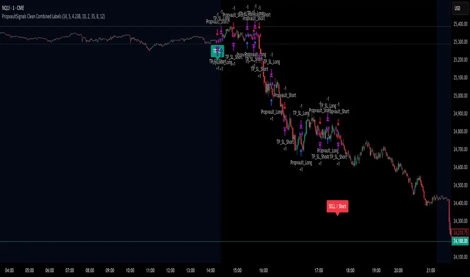
PropvaultSignals Clean Combined Labels Best Tested 91%PropvaultSignals Clean Single Label with best session
Educational
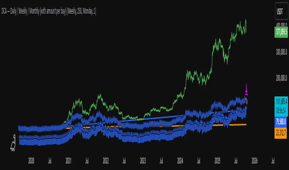
DCA Test Daily / Weekly / Monthly1.Input daily, weekly or monthly preferance of DCA
2.Select how much to DCA
3.Use the slider on the indicator down to select from where to DCA
Important: Don't use a higher timeframe chart than the desired DCA frequency, or all the DCA buys won't get executed.
DCA with the Money Supply Index DCA with the Money Supply Index (MSI) by zdmre
This strategy is based on the Money Supply Index (MSI) by zdmre and enhances it with two functional options for users: a DCA (Dollar-Cost Averaging) approach and a signal-based buy/sell mode. It’s designed to help traders and investors make data-driven, disciplined entry decisions based on monetary supply trends.
🧠 Concept Overview
The Money Supply Index (MSI) provides insight into how liquidity (money supply) influences market movements. This strategy builds upon that foundation by allowing users to either:
Accumulate positions over time using DCA, based on favorable MSI conditions.
Execute a single buy and sell trade, optimized for bull market conditions.
⚙️ Inputs Explained
General Parameters
Start Bar Index / Stop Bar Index
Defines the range of bars (historical data) for backtesting or strategy visualization.
Long DCA
Activates the DCA mode. If unchecked, the strategy operates in single-entry/single-exit signal mode.
Trading Signal
Enables signal-based entries and exits when the MSI reaches predefined thresholds.
DCA Parameters
Entry Value
The MSI value that triggers a DCA buy event. When the MSI crosses below this value, the strategy considers it a favorable moment to deploy the saved capital.
Saved Amount
The amount of money set aside regularly (e.g., monthly) for investment. This simulates the DCA effect by accumulating capital and deploying it when conditions are optimal.
Data Inputs
Money Supply
The data source for the Money Supply Index (default: ECONOMICS:USM2).
Relational Symbol
The market instrument to compare against the money supply (default: NASDAQ_DLY:NDX). This allows the strategy to measure liquidity impact on a specific market.
Chart Display Options
You can toggle these metrics on the chart for better visualization:
Entry Price (green) – The price level of executed buys.
Cash Balance (yellow) – Remaining uninvested capital.
Invested Capital (red) – Total amount currently invested.
Current Value (blue) – The current valuation of the investment.
Profit (purple) – The total realized and unrealized profit.
Trades on Chart / Signal Labels / Quantity – Enables trade markers, signal text, and position size visualization.
📈 How the Strategy Works
1️⃣ DCA Mode
In DCA mode, the strategy simulates periodic savings and only invests when the MSI indicates favorable liquidity conditions (based on the Entry Value).
This approach aims to achieve the best possible average entry price over time — a powerful strategy for long-term investors seeking stable accumulation with reduced emotional bias.
2️⃣ Signal-Based Mode
In signal mode (with DCA disabled), the strategy performs one buy and one sell trade based on MSI turning points.
It’s most effective during bull markets, where liquidity expansion supports upward momentum.
This mode helps identify high-probability entry and exit zones rather than averaging in continuously.
💡 Additional Notes
This strategy includes helpful metrics to monitor your personal investment performance — showing invested capital, cash reserves, and profit in real-time.
The goal is to combine macroeconomic insight (money supply) with disciplined execution and capital management.
⚠️ Disclaimer
This strategy is for educational and research purposes only. It does not constitute financial advice. Always conduct your own analysis before making investment decisions.

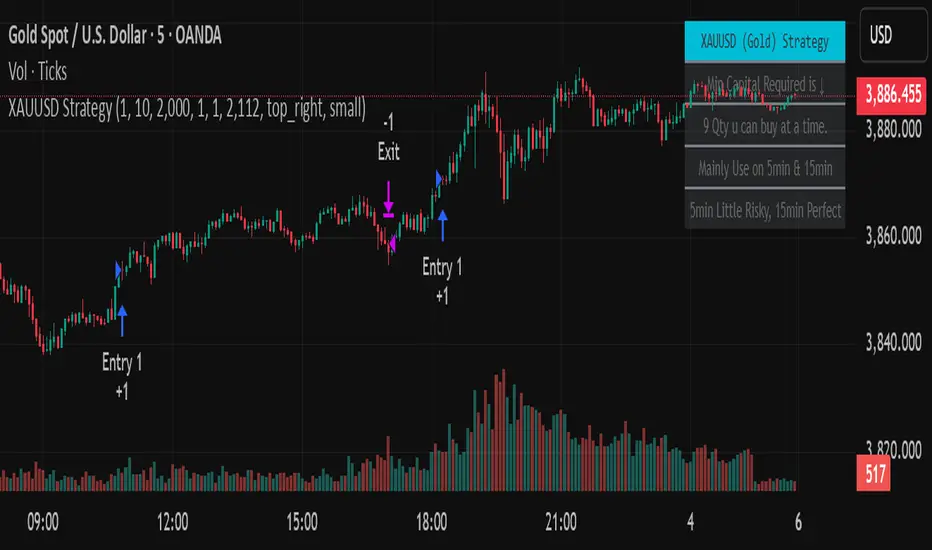
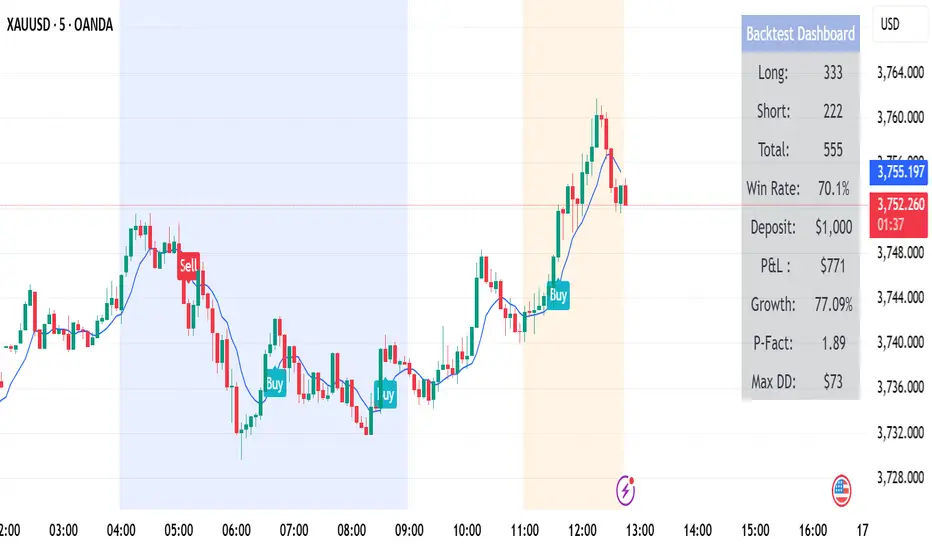
Golden StrategyTitle: XAUUSD (Gold) Smart Entry Strategy with Dynamic Scaling
Description:
This is a precision-based entry strategy for XAUUSD (Gold), optimized for lower timeframes like the 5-minute and 15-minute charts. It uses a custom logic engine to detect potential reversals and applies dynamic scaling (pyramiding) to build positions strategically based on price behavior.
🔍 Key Features:
✅ Smart entry logic for trend shifts
✅ Configurable position scaling up to 7 level
✅ Built-in capital efficiency for smaller accounts
✅ Backtest window control for historical testing
✅ Compact on-screen table for user guidance
Timeframes Recommended:
🔸 15-minute: Best balance of risk and consistency
🔸 5-minute: More frequent signals, slightly higher risk
⚠️ Important Disclaimer
This script is for educational and informational purposes only. It is not financial advice or a signal service. Trading carries risk, and past performance does not guarantee future results. Use at your own discretion and always manage risk appropriately.
Diabolos Long What the strategy tries to do
It looks for RSI dips into oversold, then waits for RSI to recover above a chosen level before placing a limit buy slightly below the current price. If the limit doesn’t fill within a few bars, it cancels it. Once in a trade, it sets a fixed take-profit and stop-loss. It can pyramid up to 3 entries.
Step-by-step
1) Inputs you control
RSI Length (rsiLen), Oversold level (rsiOS), and a re-entry threshold (rsiEntryLevel) you want RSI to reach after oversold.
Entry offset % (entryOffset): how far below the current close to place your limit buy.
Cancel after N bars (cancelAfterBars): if still not filled after this many bars, the limit order is canceled.
Risk & compounding knobs: initialRisk (% of equity for first order), compoundRate (% to artificially grow the equity base after each signal), plus fixed TP% and SL%.
2) RSI logic (arming the setup)
It calculates rsi = ta.rsi(close, rsiLen).
If RSI falls below rsiOS, it sets a flag inOversold := true (this “arms” the next potential long).
A long signal (longCondition) happens only when:
inOversold is true (we were oversold),
RSI comes back above rsiOS,
and RSI is at least rsiEntryLevel.
So: dip into OS → recover above OS and to your threshold → signal fires.
3) Placing the entry order
When longCondition is true:
It computes a limit price: close * (1 - entryOffset/100) (i.e., below the current bar’s close).
It sizes the order as positionRisk / close, where:
positionRisk starts as accountEquity * (initialRisk/100).
accountEquity was set once at script start to strategy.equity.
It places a limit long: strategy.order("Long Entry", strategy.long, qty=..., limit=limitPrice).
It then resets inOversold := false (disarms until RSI goes oversold again).
It remembers the bar index (orderBarIndex := bar_index) so it can cancel later if unfilled.
Important nuance about “compounding” here
After signaling, it does:
compoundedEquity := compoundedEquity * (1 + compoundRate/100)
positionRisk := compoundedEquity * (initialRisk/100)
This means your future order sizes grow by a fixed compound rate every time a signal occurs, regardless of whether previous trades won or lost. It’s not tied to actual PnL; it’s an artificial growth curve. Also, accountEquity was captured only once at start, so it doesn’t automatically track live equity changes.
4) Auto-cancel the limit if it doesn’t fill
On each bar, if bar_index - orderBarIndex >= cancelAfterBars, it does strategy.cancel("Long Entry") and clears orderBarIndex.
If the order already filled, cancel does nothing (there’s nothing pending with that id).
Behavioral consequence: Because you set inOversold := false at signal time (not on fill), if a limit order never fills and later gets canceled, the strategy will not fire a new entry until RSI goes below oversold again to re-arm.
5) Managing the open position
If strategy.position_size > 0, it reads the avg entry price, then sets:
takeProfitPrice = avgEntryPrice * (1 + exitGainPercentage/100)
stopLossPrice = avgEntryPrice * (1 - stopLossPercentage/100)
It places a combined exit:
strategy.exit("TP / SL", from_entry="Long Entry", limit=takeProfitPrice, stop=stopLossPrice)
With pyramiding=3, multiple fills can stack into one net long position. Using the same from_entry id ties the TP/SL to that logical entry group (not per-layer). That’s OK in TradingView (it will manage TP/SL for the position), but you don’t get per-layer TP/SL.
6) Visuals & alerts
It plots a green triangle under the bar when the long signal condition occurs.
It exposes an alert you can hook to: “Покупка при достижении уровня”.
A quick example timeline
RSI drops below rsiOS → inOversold = true (armed).
RSI rises back above rsiOS and reaches rsiEntryLevel → signal.
Strategy places a limit buy a bit below current price.
4a) If price dips to fill within cancelAfterBars, you’re long. TP/SL are set as fixed % from avg entry.
4b) If price doesn’t dip enough, after N bars the limit is canceled. The system won’t re-try until RSI becomes oversold again.
Key quirks to be aware of
Risk sizing isn’t PnL-aware. accountEquity is frozen at start, and compoundedEquity grows on every signal, not on wins. So size doesn’t reflect real equity changes unless you rewrite it to use strategy.equity each time and (optionally) size by stop distance.
Disarm on signal, not on fill. If a limit order goes stale and is canceled, the system won’t try again unless RSI re-enters oversold. That’s intentional but can reduce fills.
Single TP/SL id for pyramiding. Works, but you can’t manage each add-on with different exits.

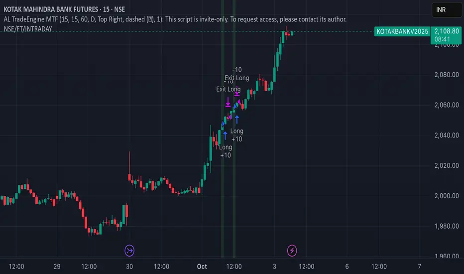
Zero Lag + Momentum Bias StrategyZero Lag + Momentum Bias Strategy (MTF + Strong MBI + R:R + Partial TP + Alerts)

NSE/FT/INTRADAYIt combines technical indicators and momentum signals to capture quick price movements while managing risk effectively. The strategy emphasizes fast execution, strict stop-loss placement, and disciplined profit booking, making it suitable for traders who prefer multiple trades within the same day rather than holding overnight positions.
Strategy Builderuse external indicators on the chart as a source for a strategy. use 5 different triggers with drop down conditions. you can use any indicator that plots.
I will amend info when I get more time. improvement suggestions or indicator combinations would be appreciated.

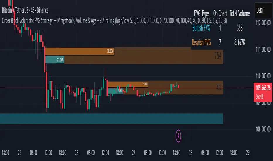
Order Block Volumatic FVG StrategyInspired by: Volumatic Fair Value Gaps —
License: CC BY-NC-SA 4.0 (Creative Commons Attribution–NonCommercial–ShareAlike).
This script is a non-commercial derivative work that credits the original author and keeps the same license.
What this strategy does
This turns BigBeluga’s visual FVG concept into an entry/exit strategy. It scans bullish and bearish FVG boxes, measures how deep price has mitigated into a box (as a percentage), and opens a long/short when your mitigation threshold and filters are satisfied. Risk is managed with a fixed Stop Loss % and a Trailing Stop that activates only after a user-defined profit trigger.
Additions vs. the original indicator
✅ Strategy entries based on % mitigation into FVGs (long/short).
✅ Lower-TF volume split using upticks/downticks; fallback if LTF data is missing (distributes prior bar volume by close’s position in its H–L range) to avoid NaN/0.
✅ Per-FVG total volume filter (min/max) so you can skip weak boxes.
✅ Age filter (min bars since the FVG was created) to avoid fresh/immature boxes.
✅ Bull% / Bear% share filter (the 46%/53% numbers you see inside each FVG).
✅ Optional candle confirmation and cooldown between trades.
✅ Risk management: fixed SL % + Trailing Stop with a profit trigger (doesn’t trail until your trigger is reached).
✅ Pine v6 safety: no unsupported args, no indexof/clamp/when, reverse-index deletes, guards against zero/NaN.
How a trade is decided (logic overview)
Detect FVGs (same rules as the original visual logic).
For each FVG currently intersected by the bar, compute:
Mitigation % (how deep price has entered the box).
Bull%/Bear% split (internal volume share).
Total volume (printed on the box) from LTF aggregation or fallback.
Age (bars) since the box was created.
Apply your filters:
Mitigation ≥ Long/Short threshold.
Volume between your min and max (if enabled).
Age ≥ min bars (if enabled).
Bull% / Bear% within your limits (if enabled).
(Optional) the current candle must be in trade direction (confirm).
If multiple FVGs qualify on the same bar, the strategy uses the most recent one.
Enter long/short (no pyramiding).
Exit with:
Fixed Stop Loss %, and
Trailing Stop that only starts after price reaches your profit trigger %.
Input settings (quick guide)
Mitigation source: close or high/low. Use high/low for intrabar touches; close is stricter.
Mitigation % thresholds: minimal mitigation for Long and Short.
TOTAL Volume filter: skip FVGs with too little/too much total volume (per box).
Bull/Bear share filter: require, e.g., Long only if Bull% ≥ 50; avoid Short when Bull% is high (Short Bull% max).
Age filter (bars): e.g., ≥ 20–30 bars to avoid fresh boxes.
Confirm candle: require candle direction to match the trade.
Cooldown (bars): minimum bars between entries.
Risk:
Stop Loss % (fixed from entry price).
Activate trailing at +% profit (the trigger).
Trailing distance % (the trailing gap once active).
Lower-TF aggregation:
Auto: TF/Divisor → picks 1/3/5m automatically.
Fixed: choose 1/3/5/15m explicitly.
If LTF can’t be fetched, fallback allocates prior bar’s volume by its close position in the bar’s H–L.
Suggested starting presets (you should optimize per market)
Mitigation: 60–80% for both Long/Short.
Bull/Bear share:
Long: Bull% ≥ 50–70, Bear% ≤ 100.
Short: Bull% ≤ 60 (avoid shorting into strong support), Bear% ≥ 0–70 as you prefer.
Age: ≥ 20–30 bars.
Volume: pick a min that filters noise for your symbol/timeframe.
Risk: SL 4–6%, trailing trigger 1–2%, distance 1–2% (crypto example).
Set slippage/fees in Strategy Properties.
Notes, limitations & best practices
Data differences: The LTF split uses request.security_lower_tf. If the exchange/data feed has sparse LTF data, the fallback kicks in (it’s deliberate to avoid NaNs but is a heuristic).
Real-time vs backtest: The current bar can update until close; results on historical bars use closed data. Use “Bar Replay” to understand intrabar effects.
No pyramiding: Only one position at a time. Modify pyramiding in the header if you need scaling.
Assets: For spot/crypto, TradingView “volume” is exchange volume; in some markets it may be tick volume—interpret filters accordingly.
Risk disclosure: Past performance ≠ future results. Use appropriate position sizing and risk controls; this is not financial advice.
Credits
Visual FVG concept and original implementation: BigBeluga.
This derivative strategy adds entry/exit logic, volume/age/share filters, robust LTF handling, and risk management while preserving the original spirit.
License remains CC BY-NC-SA 4.0 (non-commercial, attribution required, share-alike).
KD The ScalperWe have to take the trade when all three EMAs are pointing in the same direction (no criss-cross, no up/down, sideways). All 3 EMAs should be cleanly separated from each other with strong spacing between them; they are not tangled, sideways, or messy. This is our first filter before entering the trade. Are the EMAs stacked neatly, and is the price outside of the 25 EMA? If price pulls back and closes near or below the 25 or 50 EMA and breaks the 100 EMA, we don't trade. Use the 100 EMA as a safety net and refrain from trading if the price touches or falls below the 100 EMA.
1. Confirm the trend- All 3 EMAs must align, and they must spread
2. Watch price pull back to the 25th or the 50 EMA
3. Wait for the price to bounce - And re-approach the 25 EMA
Why is this powerful?
Removes 80% of the low-probability Trades
It keeps you out of choppy markets
Avoids Reversal Traps
Anchors us to momentum
We take the entry when the price moves up again and touches the 25 EMA from below, and then when it breaks above the 25 EMA, or even better, when a lovely green bullish candle forms. A bullish candle indicates good momentum. When a bullish candle closes in green, it means the momentum has increased significantly. This is when we enter a long trade, with the stop-loss just below the 50 EMA and the profit target being 1.5 times the stop-loss.
The same rule applies to the bearish trade.

G. Santostasi Bitcoin Power Law StrategyG. Santostasi Bitcoin Power Law Strategy
Overview
The "G. Santostasi Bitcoin Power Law Strategy" is a TradingView strategy script built upon the foundational Bitcoin Power Law Theory by physicist Giovanni Santostasi.
Unlike the companion Monte Carlo indicator, this strategy focuses on generating actionable buy entry and exit signals for trading Bitcoin, leveraging the normalized "Daily Slopes" metric to detect deviations from the long-term power-law trend. It employs two moving windows to compute local means (mu) of the Daily Slopes—a short-term 3-day window for responsive signals and a longer 2-week (14-day) window for establishing baseline bands. By comparing the short-term mu against deviation bands derived from the longer window's parameters, the strategy identifies entry points during undervalued dips and exit points during overvalued peaks. This approach capitalizes on Bitcoin's scale-invariant behavior, where price follows a power law
P(t)= c t^n, with n~5.9.
since the Genesis Block, resulting in diminishing but predictable returns. Backtested over Bitcoin's full history, the strategy boasts a 77% winning rate and a profit factor of 3.2, making it a robust tool for trend-following with mean-reversion elements. It emphasizes Bitcoin's long-term stability while navigating short-term oscillations, treating cycles as temporary deviations from the core power-law "DNA.
"Core Concept: Daily Slopes
The strategy inherits the Daily Slopes metric from the power-law framework, which normalizes daily logarithmic returns to reveal a stable local slope that oscillates around the global value of ~5.9.Definition and Calculation:
Daily log returns: log(P2/P1)\, where P2 and P1 are consecutive closing prices.
Normalization: Divide by log((t+1)/t), where ( t ) is days since the Genesis Block, yielding:
Daily Slope=log(P2/P1)log((t+1)/t).
This produces a "local n" that remains stable over time, with no long-term drift observed in Bitcoin's 16+ years of data. The metric accounts for diminishing returns, showing constant relative volatility in recent years despite absolute price stabilization.
Distribution and Parameters:
Daily Slopes are fitted to a t-location scale distribution over moving windows, estimating:μ (mu): The location/mean, stable around 5.9 globally.
σ (sigma): Scale/volatility measure.
ν (nu): Degrees of freedom for tail heaviness.
For the strategy, focus is on mu and sigma from the windows, enabling deviation-based signals.
Strategy Logic: Dual Moving Window Mus and Deviation Bands
The strategy computes two mus via rolling fits to the t-distribution:
Short Window mu (3 days): A fast-moving average of Daily Slopes, sensitive to immediate price action for timely signals.
Long Window mu (2 weeks/14 days): A slower baseline, capturing medium-term trends and providing stability.
Deviation bands are derived from the long window's mu and sigma:
Upper Band: Long mu + Long sigma
Lower Band: Long mu - Long sigma
These bands represent 1-standard-deviation ranges around the longer-term mean, highlighting overbought and oversold conditions relative to the power-law trend. The short mu acts as a "signal line," crossing the bands to trigger trades.
Plotting:
Short mu: Responsive line for crossovers.
Long mu: Central baseline.
Bands: Upper (+σ) and lower (-σ) lines from the long window.
Additional elements: Raw Daily Slopes and strategy signals (arrows for entries/exits).
Entry and Exit Rules:
The strategy generates long-only signals (buy/sell) based on crossovers, assuming a single-position approach without leverage or shorting:
Buy Entry: Triggered when the short-window mu crosses above the lower band (long mu - long sigma). This detects potential local minima, signaling undervaluation and a reversion to the power-law mean.
Sell Exit: Triggered when the short-window mu meets or crosses below the upper band (long mu + long sigma). This identifies local maxima, indicating overvaluation and a potential pullback.
Trade Management:
No stop-loss or take-profit hardcoded; users can add via TradingView settings.
Positions close on exit signals, with re-entry on the next valid buy.
Filters for false signals: Optional confirmation from global slope (e.g., only trade if long mu > 5.0) to align with bullish regimes.
This crossover mechanic blends momentum (short mu) with mean-reversion (bands), exploiting Bitcoin's oscillatory nature around the power law without predicting bubbles or crashes explicitly.
Performance Metrics:
Backtested on BTCUSD daily data from the Genesis Block to present (assuming continuous updates):Winning Rate: 77% – A high hit rate due to the strategy's focus on statistically stable deviations.
Profit Factor: 3.2 – Gross profits are 3.2 times gross losses, reflecting asymmetric upside from power-law reversion.
Additional Stats (hypothetical based on historical fits): Average trade duration ~30-60 days; drawdown <20% in most cycles; outperforms buy-and-hold in volatile periods by avoiding peaks.
Caveats: Past performance is not indicative of future results. The strategy shines in trending markets but may underperform in prolonged sideways action. Transaction costs (e.g., fees, slippage) not included in base metrics.
Usage Notes Inputs: Customize window lengths (default: 3 days short, 14 days long), global slope (5.9), and signal thresholds. Enable alerts for entries/exits.
Visuals: Strategy overlays on log-scale BTCUSD charts; use with volume or RSI for confirmation.
Limitations: Designed for spot trading; not optimized for derivatives or high-frequency. Assumes power-law persistence—major regime shifts (e.g., adoption plateaus) could impact efficacy.
Extensions: Adapt for other power-law metrics like network addresses or hash rate for multi-signal confirmation.
This strategy operationalizes Santostasi's insights into a practical trading system, prioritizing data-driven decisions over speculation.

AR Alerts Basic 🤖A non-repainting, ATR-based trailing stop strategy and session-based trading filters.
Features:
Dynamic buy/sell trailing stops using ATR for stable exits.
EMA exit for remaining positions to lock in profits.
Time session filters: trade only during defined market hours.
Trend detection using EMA50/EMA100 coloring.
Backtest dashboard Table showing total trades, win rate, P&L, growth, profit factor, and max drawdown. can be uncheck from Style Tab.
Fully non-repainting signals for reliable historical testing.
Perfect for traders who want stable signals, trailing stops, and a clean backtest summary in one indicator.
@infonatics
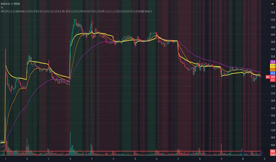
AVGO Advanced Day Trading Strategy📈 Overview
The AVGO Advanced Day Trading Strategy is a comprehensive, multi-timeframe trading system designed for active day traders seeking consistent performance with robust risk management. Originally optimized for AVGO (Broadcom), this strategy adapts well to other liquid stocks and can be customized for various trading styles.
🎯 Key Features
Multiple Entry Methods
EMA Crossover: Classic trend-following signals using fast (9) and medium (16) EMAs
MACD + RSI Confluence: Momentum-based entries combining MACD crossovers with RSI positioning
Price Momentum: Consecutive price action patterns with EMA and RSI confirmation
Hybrid System: Advanced multi-trigger approach combining all methodologies
Advanced Technical Arsenal
When enabled, the strategy analyzes 8+ additional indicators for confluence:
Volume Price Trend (VPT): Measures volume-weighted price momentum
On-Balance Volume (OBV): Tracks cumulative volume flow
Accumulation/Distribution Line: Identifies institutional money flow
Williams %R: Momentum oscillator for entry timing
Rate of Change Suite: Multi-timeframe momentum analysis (5, 14, 18 periods)
Commodity Channel Index (CCI): Cyclical turning points
Average Directional Index (ADX): Trend strength measurement
Parabolic SAR: Dynamic support/resistance levels
🛡️ Risk Management System
Position Sizing
Risk-based position sizing (default 1% per trade)
Maximum position limits (default 25% of equity)
Daily loss limits with automatic position closure
Multiple Profit Targets
Target 1: 1.5% gain (50% position exit)
Target 2: 2.5% gain (30% position exit)
Target 3: 3.6% gain (20% position exit)
Configurable exit percentages and target levels
Stop Loss Protection
ATR-based or percentage-based stop losses
Optional trailing stops
Dynamic stop adjustment based on market volatility
📊 Technical Specifications
Primary Indicators
EMAs: 9 (Fast), 16 (Medium), 50 (Long)
VWAP: Volume-weighted average price filter
RSI: 6-period momentum oscillator
MACD: 8/13/5 configuration for faster signals
Volume Confirmation
Volume filter requiring 1.6x average volume
19-period volume moving average baseline
Optional volume confirmation bypass
Market Structure Analysis
Bollinger Bands (20-period, 2.0 multiplier)
Squeeze detection for breakout opportunities
Fractal and pivot point analysis
⏰ Trading Hours & Filters
Time Management
Configurable trading hours (default: 9:30 AM - 3:30 PM EST)
Weekend and holiday filtering
Session-based trade management
Market Condition Filters
Trend alignment requirements
VWAP positioning filters
Volatility-based entry conditions
📱 Visual Features
Information Dashboard
Real-time display of:
Current entry method and signals
Bullish/bearish signal counts
RSI and MACD status
Trend direction and strength
Position status and P&L
Volume and time filter status
Chart Visualization
EMA plots with customizable colors
Entry signal markers
Target and stop level lines
Background color coding for trends
Optional Bollinger Bands and SAR display
🔔 Alert System
Entry Alerts
Customizable alerts for long and short entries
Method-specific alert messages
Signal confluence notifications
Advanced Alerts
Strong confluence threshold alerts
Custom alert messages with signal counts
Risk management alerts
⚙️ Customization Options
Strategy Parameters
Enable/disable long or short trades
Adjustable risk parameters
Multiple entry method selection
Advanced indicator on/off toggle
Visual Customization
Color schemes for all indicators
Dashboard position and size options
Show/hide various chart elements
Background color preferences
📋 Default Settings
Initial Capital: $100,000
Commission: 0.1%
Default Position Size: 10% of equity
Risk Per Trade: 1.0%
RSI Length: 6 periods
MACD: 8/13/5 configuration
Stop Loss: 1.1% or ATR-based
🎯 Best Use Cases
Day Trading: Designed for intraday opportunities
Swing Trading: Adaptable for longer-term positions
Momentum Trading: Excellent for trending markets
Risk-Conscious Trading: Built-in risk management protocols
⚠️ Important Notes
Paper Trading Recommended: Test thoroughly before live trading
Market Conditions: Performance varies with market volatility
Customization: Adjust parameters based on your risk tolerance
Educational Purpose: Use as a learning tool and customize for your needs
🏆 Performance Features
Detailed performance metrics
Trade-by-trade analysis capability
Customizable risk/reward ratios
Comprehensive backtesting support
This strategy is for educational purposes. Past performance does not guarantee future results. Always practice proper risk management and consider your financial situation before trading.
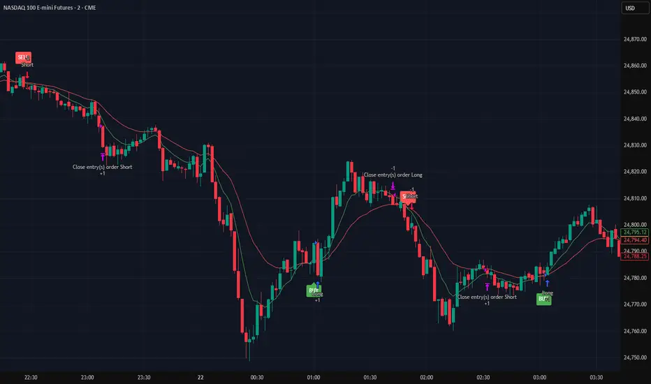
Alpha SignalsThis strategy is designed to highlight potential short-term market setups using a fast and slow EMA crossover system on a 5-minute chart. It provides visual signals directly on the chart to help traders observe trend changes and potential entry points.
Key Features:
EMA Crossover Entries – The strategy enters long trades when the fast EMA crosses above the slow EMA and short trades when the fast EMA crosses below the slow EMA.
Time-Based Exits – Trades are automatically closed after a configurable number of bars to manage exposure.
Visual Alerts – Buy and sell signals are displayed as labels directly on the chart for easy interpretation.
Configurable Settings – Users can adjust fast and slow EMA lengths as well as the exit bar count to suit their trading preferences.
Usage:
Suitable for short-term traders focusing on the NQ1 futures contract or other instruments with similar volatility.
Can be used for observation, back testing, or as a confirmation tool alongside other strategies.
Does not guarantee profitability; intended for educational purposes and strategy testing only.
EMA 8/33 Optimized Crossover w/FilterThis strategy is ideal for fast-moving assets like cryptocurrencies (e.g., SOLUSDT) on intraday to swing trading timeframes. Its robust filtering aims for fewer trades but with higher accuracy, producing a smoother equity curve and lower drawdown in your backtests.
You can further optimize the EMA lengths, minimum candle size, and TP/SL percentages to suit your preferred asset and timeframe.

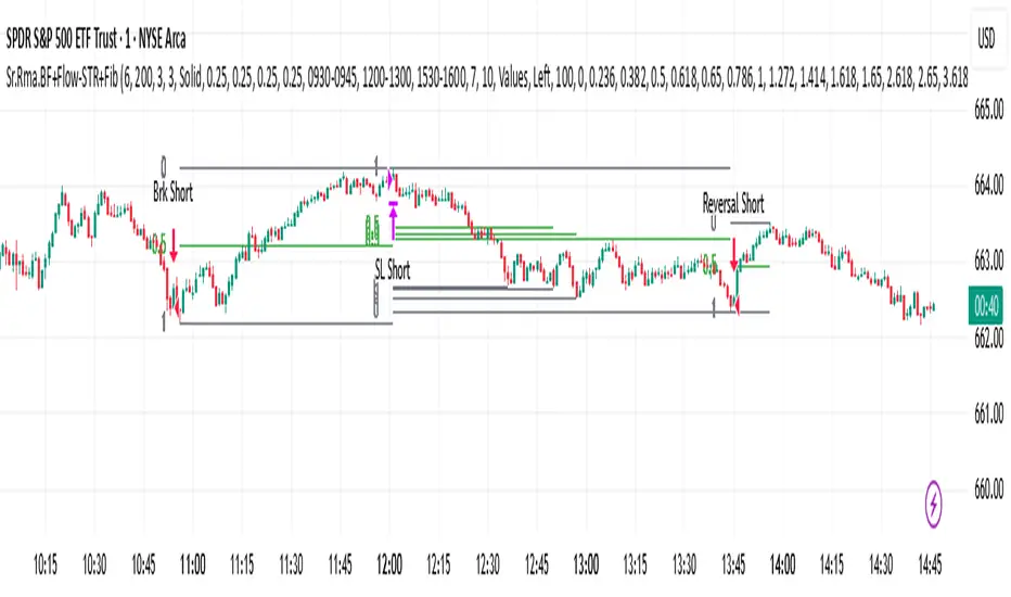
Sr.Rma.Breakout.Fib (Merged)DO YOUR DUE DILIGENCE – THIS IS FOR EDUCATIONAL PURPOSE AND NOT A TRADE ADVICE-
This strategy is designed for traders who want to merge pattern recognition (breakouts) with market structure context (Fibonacci), while maintaining disciplined trade management through automated stop-loss and reversal logic. “Once the chart is added, please ensure the candle pattern is set to Heikin Ashi.”
1. Breakout Finder Logic
The breakout finder identifies bullish and bearish breakouts using pivots, thresholds, and test counts:
• Pivot Highs & Lows (PH/PL): Calculated using user-defined periods.
• Breakout Threshold: Dynamic channel width based on recent volatility.
• Confirmation: A breakout is validated when price action clears the breakout Conditions
• Bullish Breakout: Triggered when multiple pivot highs are cleared by bullish Conditions.
• Bearish Breakout: Triggered when multiple pivot lows are broken by bearish Conditions.
• Sessions ignored: Traders can exclude up to three custom time windows to prevent signals during low-quality periods.
Risk & Reversal Controls
• Stop-Loss: Adjustable % thresholds for both long and short trades.
• Reversal Entries: Optional signals that trigger after a stop-loss, capturing potential price reversals.
2. Strategy Order Management
The strategy executes entries and exits based on confirmed breakout and reversal signals:
• Entries:
o Long on confirmed bullish breakout.
o Short on confirmed bearish breakout.
• Stops:
o Automatic closure of open positions when stop-loss conditions are hit.
• Reversals:
o Transition directly from long to short or vice versa when reversal conditions are met.
3. Auto Fibonacci Retracement
A ZigZag-based system automatically plots Fibonacci retracement levels on the chart:
• Swing Context: Derived dynamically from pivots with adjustable depth and deviation settings.
• Fib Levels: Standard retracement and extension levels (0.236, 0.382, 0.5, 0.618, 0.786, 1.0, 1.618, 2.618, 3.618, 4.236, etc.) are supported.
• Custom Options:
o Extend lines left or right.
o Show/hide level prices and percentage values.
o Control label positions (left or right).
o Adjustable transparency for background fills between levels.
• Crossing Alerts: Alerts are fired when the price crosses specific Fibonacci levels, enhancing confluence with breakout signals.
5. Key Benefits
• Comprehensive Trading Framework: Combines breakout confirmation, risk management, and Fibonacci context.
• Visual Clarity: Automatic plotting of breakout structures and Fib levels makes the chart intuitive.
• Flexible Controls: Full customization of pivots, thresholds, sessions, stop-loss %, and Fib settings.
• Automation Ready: Alerts and strategy orders allow seamless integration with brokers or external systems.
MOONA130925-2305bThe Martingale strategy in crypto trading involves doubling trade size after each loss, aiming to recover losses with one win and secure a small profit. While potentially effective short-term, it carries high risk, as consecutive losses can rapidly exhaust capital, making it unsustainable without strict risk management.
Use Below Settings for Best Results.
5Min or 15 Min
EMA 20
EMA 45
EMA 200
Keep Enable EMA on Entry- ON
Length 1- 45
Length 2- 200
Set Target 3% (Untick all Except T1)
Set SL 1.5%

Sr.Ram.GodSoun.Market StructureDisclaimer: This chart is for educational purposes only. Please do your own due diligence — this is not trade advice. Any signals for buys, sells, calls, or puts are purely strategy outputs and should not be considered trading recommendations.
This strategy is designed for "SPY" and "QQQ" on a 3-minute time frame. It is built on market-structure breakouts, identifying swing highs and lows using a configurable Market Structure Duration.
A bullish breakout triggers a Calls (long) entry, while a bearish breakout triggers a Puts (short) entry.
Signals are filtered with session-based exclusions, ensuring no entries or exits occur during the following EST time windows:
09:30 – 09:45
12:00 – 13:00
15:30 – 16:00
Risk management is enforced through percentage-based exits:
Close Longs and switch to Puts if price moves 0.2%
Close Puts and switch to Calls if price moves 0.2%
The strategy also incorporates re-entry logic after a stop-out:
Re-enter Puts on a further 0.3% breakdown.
Re-enter Calls on a further 0.3% breakout.
Built-in alerts cover all entries, exits, and re-entries, enabling seamless use with automated trading or notifications.

Sr.Rma.Prev High/lows with Alerts
Disclaimer: This chart is designed for educational purposes only. Please conduct your own due diligence before entering any trades.
The strategy is based on previous highs and lows, combined with stop-loss and reversal percentage logic. It is most effective on SPY and QQQ using the 1-minute time-frame, where I personally trade next-day expiration with preset configurations.
If you choose to apply it to other stocks, be sure to adjust the stop-loss % and re-entry % parameters to match your trading style and risk tolerance.

Trade Stock One v3Professional Trading Strategy
Specializes in trading uptrends, riding long-term waves
Limits frequent entries
Suitable for medium- to long-term stock trading

Ajay Nayak - EMA ATR Trailinge strategy RSI aur RSI ke SMA ke crossover par CALL aur PUT signal generate karti hai.
Saath me ATR based stoploss aur crossover target bhi diya gaya hai.
Algo trading ke liye useful hai.

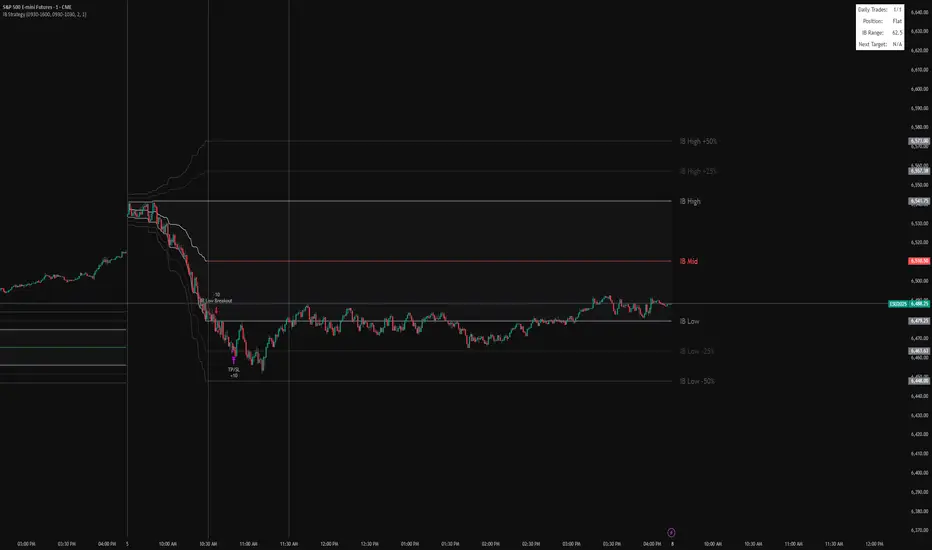
IB BreakoutIt marks the IB range (high, low, midpoint) from a chosen session window (default 9:30–10:30).
It plots the IB lines, midpoint (colored based on close), and extension levels (+/–25% and 50%).
After the IB session ends, it looks for breakouts:
Long if price closes above IB high.
Short if price closes below IB low.
Each trade targets the 25% extension in the breakout direction, with an optional stop at the opposite IB level.
It limits the number of trades per day and displays info (trades, position, IB range, next target) in a table.
LFT strategy Main Reversion
this script will tell exactly when to buy and sell with TP and SL, used the latest LLM to tone the model with a profit ratio of 2.05 in 6 years and profit ratio of 4.02 in past 6 month and have been back tested with Monte Carlo simulation, with profit ratio 1+ for 99% of the time with 1000 iterations with 500 steps, for 100 times
please contact LFT Foundation for access
