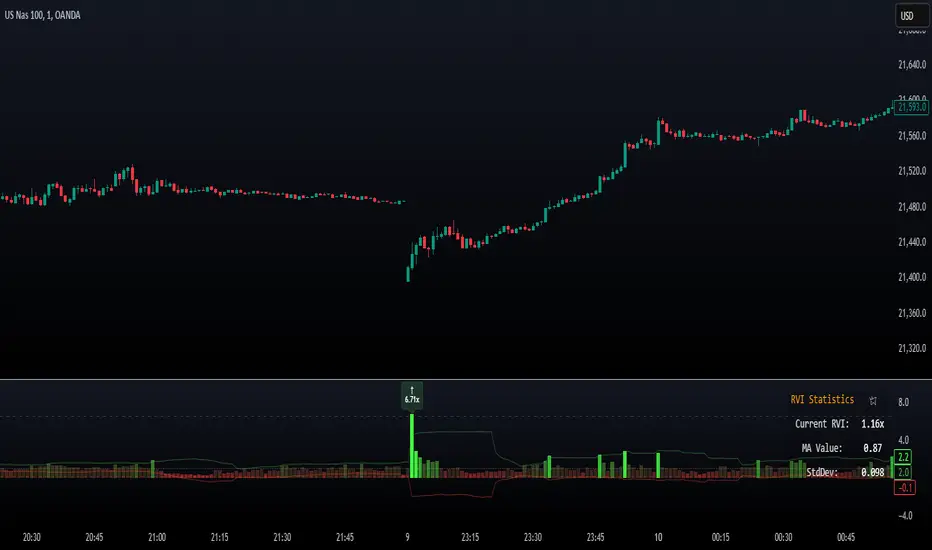
Relative Volume Index [PhenLabs]Relative Volume Index (RVI)
Version: PineScript™ v6
Description
The Relative Volume Index (RVI) is a sophisticated volume analysis indicator that compares real-time trading volume against historical averages for specific time periods. By analyzing volume patterns and statistical deviations, it helps traders identify unusual market activity and potential trading opportunities. The indicator uses dynamic color visualization and statistical overlays to provide clear, actionable volume analysis.
Components
• Volume Comparison: Real-time volume relative to historical averages
• Statistical Bands: Upper and lower deviation bands showing volume volatility
• Moving Average Line: Smoothed trend of relative volume
• Color Gradient Display: Visual representation of volume strength
• Statistics Dashboard: Real-time metrics and calculations
Usage Guidelines
Volume Strength Analysis:
• Values > 1.0 indicate above-average volume
• Values < 1.0 indicate below-average volume
• Watch for readings above the threshold (default 6.5x) for exceptional volume
Trading Signals:
• Strong volume confirms price moves
• Divergences between price and volume suggest potential reversals
• Use extreme readings as potential reversal signals
Optimal Settings:
• Start with default 15-bar lookback for general analysis
• Adjust threshold (6.5x) based on market volatility
• Use with multiple timeframes for confirmation
Best Practices:
• Combine with price action and other indicators
• Monitor deviation bands for volatility expansion
• Use the statistics panel for precise readings
• Pay attention to color gradients for quick assessment
Limitations
• Requires quality volume data for accurate calculations
• May produce false signals during pre/post market hours
• Historical comparisons may be skewed during unusual market conditions
• Best suited for liquid markets with consistent volume patterns
Note: For optimal results, use in conjunction with price action analysis and other technical indicators. The indicator performs best during regular market hours on liquid instruments.
Biến động Lịch sử
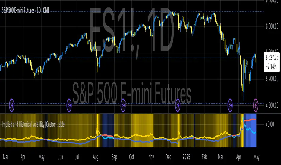
Implied and Historical VolatilityAbstract
This TradingView indicator visualizes implied volatility (IV) derived from the VIX index and historical volatility (HV) computed from past price data of the S&P 500 (or any selected asset). It enables users to compare market participants' forward-looking volatility expectations (via VIX) with realized past volatility (via historical returns). Such comparisons are pivotal in identifying risk sentiment, volatility regimes, and potential mispricing in derivatives.
Functionality
Implied Volatility (IV):
The implied volatility is extracted from the VIX index, often referred to as the "fear gauge." The VIX represents the market's expectation of 30-day forward volatility, derived from options pricing on the S&P 500. Higher values of VIX indicate increased uncertainty and risk aversion (Whaley, 2000).
Historical Volatility (HV):
The historical volatility is calculated using the standard deviation of logarithmic returns over a user-defined period (default: 20 trading days). The result is annualized using a scaling factor (default: 252 trading days). Historical volatility represents the asset's past price fluctuation intensity, often used as a benchmark for realized risk (Hull, 2018).
Dynamic Background Visualization:
A dynamic background is used to highlight the relationship between IV and HV:
Yellow background: Implied volatility exceeds historical volatility, signaling elevated market expectations relative to past realized risk.
Blue background: Historical volatility exceeds implied volatility, suggesting the market might be underestimating future uncertainty.
Use Cases
Options Pricing and Trading:
The disparity between IV and HV provides insights into whether options are over- or underpriced. For example, when IV is significantly higher than HV, options traders might consider selling volatility-based derivatives to capitalize on elevated premiums (Natenberg, 1994).
Market Sentiment Analysis:
Implied volatility is often used as a proxy for market sentiment. Comparing IV to HV can help identify whether the market is overly optimistic or pessimistic about future risks.
Risk Management:
Institutional and retail investors alike use volatility measures to adjust portfolio risk exposure. Periods of high implied or historical volatility might necessitate rebalancing strategies to mitigate potential drawdowns (Campbell et al., 2001).
Volatility Trading Strategies:
Traders employing volatility arbitrage can benefit from understanding the IV/HV relationship. Strategies such as "long gamma" positions (buying options when IV < HV) or "short gamma" (selling options when IV > HV) are directly informed by these metrics.
Scientific Basis
The indicator leverages established financial principles:
Implied Volatility: Derived from the Black-Scholes-Merton model, implied volatility reflects the market's aggregate expectation of future price fluctuations (Black & Scholes, 1973).
Historical Volatility: Computed as the realized standard deviation of asset returns, historical volatility measures the intensity of past price movements, forming the basis for risk quantification (Jorion, 2007).
Behavioral Implications: IV often deviates from HV due to behavioral biases such as risk aversion and herding, creating opportunities for arbitrage (Baker & Wurgler, 2007).
Practical Considerations
Input Flexibility: Users can modify the length of the HV calculation and the annualization factor to suit specific markets or instruments.
Market Selection: The default ticker for implied volatility is the VIX (CBOE:VIX), but other volatility indices can be substituted for assets outside the S&P 500.
Data Frequency: This indicator is most effective on daily charts, as VIX data typically updates at a daily frequency.
Limitations
Implied volatility reflects the market's consensus but does not guarantee future accuracy, as it is subject to rapid adjustments based on news or events.
Historical volatility assumes a stationary distribution of returns, which might not hold during structural breaks or crises (Engle, 1982).
References
Black, F., & Scholes, M. (1973). "The Pricing of Options and Corporate Liabilities." Journal of Political Economy, 81(3), 637-654.
Whaley, R. E. (2000). "The Investor Fear Gauge." The Journal of Portfolio Management, 26(3), 12-17.
Hull, J. C. (2018). Options, Futures, and Other Derivatives. Pearson Education.
Natenberg, S. (1994). Option Volatility and Pricing: Advanced Trading Strategies and Techniques. McGraw-Hill.
Campbell, J. Y., Lo, A. W., & MacKinlay, A. C. (2001). The Econometrics of Financial Markets. Princeton University Press.
Jorion, P. (2007). Value at Risk: The New Benchmark for Managing Financial Risk. McGraw-Hill.
Baker, M., & Wurgler, J. (2007). "Investor Sentiment in the Stock Market." Journal of Economic Perspectives, 21(2), 129-151.
Machine Learning RSI Bands V3The Machine Learning RSI Bands V3 is a cutting-edge trading tool designed to provide actionable insights by combining the strength of machine learning with a traditional RSI framework. It adapts dynamically to changing market conditions, offering traders a robust, data-driven approach to identifying opportunities.
Let’s break down its functionality and the logic behind each input to give you a clear understanding of how it works and how you can use it effectively.
RSI Parameters RSI Source (rsisrc): Choose the data source for RSI calculation, such as the closing price. This allows you to focus on the specific price data that aligns with your trading strategy. RSI Length (rsilen): Set the number of periods used for RSI calculation. A shorter length makes the RSI more reactive to price changes, while a longer length smooths out volatility. These inputs allow you to customize the foundational RSI calculations, ensuring the indicator fits your style of trading.
Band Limits Lower Band Limit (lb): Defines the RSI value below which the market is considered oversold. Upper Band Limit (ub): Defines the RSI value above which the market is considered overbought. These settings give you control over the thresholds for market conditions. By adjusting the band limits, you can tailor the indicator to be more or less sensitive to market movements.
Sampling and Reaction Settings Target Reaction Size (l): Determines the number of bars used to define pivot points. Smaller values react to shorter-term price movements, while larger values focus on broader trends. Backtesting Reaction Size (btw): Sets the number of bars used to validate signal performance. This ensures signals are only considered valid if they perform consistently within the specified range. Data Format (version): Choose between Absolute (ignoring direction) and Directional (incorporating directional price changes). Sampling Method (sm): Select how the data is analyzed—options include Price Movement, Volume Movement, RSI Movement, Trend Movement, or a Hybrid approach. These settings empower you to refine how the indicator processes and interprets data, whether focusing on short-term price shifts or broader market trends.
Signal Settings Signal Confidence Method (cm): Choose between: Threshold: Signals must meet a confidence limit before being generated. Voting: Requires a majority of 5 signal components to confirm a trade. Confidence Limit (cl): Defines the confidence threshold for generating signals when using the Threshold method. Votes Needed (vn): Sets the number of votes required to confirm a trade when using the Voting method. Use All Outputs (fm): If enabled, signals are generated without filtering, providing an unfiltered view of potential opportunities. This section offers a balance between precision and flexibility, enabling you to control the rigor applied to signal generation.
How It Works
The script uses machine learning models to adaptively calculate dynamic RSI bands. These bands adjust based on market conditions, providing a more responsive and nuanced interpretation of overbought and oversold levels.
Dynamic Bands: The lower and upper RSI bands are recalibrated using machine learning to reflect current market conditions. Signals: Long and short signals are generated when RSI crosses these bands, with additional filters applied based on your chosen confidence method and sampling settings. Transparency: Real-time success rates and profit factors are displayed on the chart, giving you clear feedback on the indicator's performance.
Why Use Machine Learning RSI Bands V3?
This indicator is built for traders who want more than static thresholds and generic signals. It offers:
Adaptability: Machine learning dynamically adjusts the indicator to market conditions. Customizability: Each input serves a specific purpose, giving you full control over its behavior. Accountability: With built-in performance metrics, you always know how the tool is performing.
This is a tool designed for those who value precision and adaptability in trading.

Ultra Volume High Breakoutser Inputs:
length: Defines the period to calculate the moving average of volume.
multiplier: Sets the threshold above the moving average to consider as "Ultra Volume."
breakoutMultiplier: Allows for customization of breakout sensitivity.
Volume Calculation:
The script calculates a simple moving average (SMA) of the volume for a defined period (length).
It then detects if the current volume is higher than the moving average multiplied by the user-defined multiplier.
Breakout Condition:
The script checks if the price has moved above the highest close of the previous length periods while the volume condition for "Ultra Volume" is true.
Visuals:
The script marks the breakout with an upward label below the bar (plotshape), colored green for easy identification.
Ultra volume is highlighted with a red histogram plot.
Alert Condition:
An alert condition is included to trigger whenever an ultra volume high breakout occurs.
Customization:
You can adjust the length, multiplier, and breakoutMultiplier to fit your strategy and asset volatility.
Alerts can be set in TradingView to notify you when this condition is met.
Let me know if you'd like further customization or explanation!

Hourly Change Table (UTC Adjustable)### Indicator Description: Hourly Change Table (UTC Adjustable)
The **Hourly Change Table (UTC Adjustable)** is a powerful tool designed for analyzing **hourly average price changes** across financial instruments. By calculating and sorting these averages, the indicator identifies the hours with the most significant positive and negative price movements. It also provides visual highlights directly on the chart for easier decision-making.
---
### What Does This Indicator Do?
1. **Analyzes Hourly Average Price Changes**:
- It calculates the **average percentage price change** for each hour based on the selected lookback period.
2. **Displays a Ranked Table**:
- The indicator generates a table ranking hourly averages from the highest to the lowest, allowing you to see which hours are the most impactful.
3. **Highlights Max and Min Hours on the Chart**:
- The hour with the highest average price change is highlighted in **green**.
- The hour with the lowest average price change is highlighted in **red**.
4. **Adjusts for Time Zones**:
- A customizable **UTC Offset** ensures the indicator aligns with your preferred time zone.
---
### Key Features
1. **Customizable Lookback Period**:
- Define how many bars the indicator analyzes to calculate meaningful trends.
2. **Time Zone Adjustment**:
- Adjust the UTC offset to match your local trading hours or preferred analysis window.
3. **Graphical Chart Highlights**:
- Instantly identify the most significant hours with color-coded chart backgrounds.
4. **Sorted Data Table**:
- View a ranked list of hourly averages with the maximum and minimum values highlighted for quick reference.
---
### How to Use This Indicator?
1. **Add to Your Chart**:
- Apply the indicator to any financial instrument and time frame on TradingView.
2. **Set the Lookback Period**:
- Configure the "Lookback Bars" setting to define how many bars the indicator should analyze.
3. **Configure the UTC Offset**:
- Align the indicator with your preferred time zone by setting the appropriate UTC offset (e.g., `2` for UTC+2).
4. **Enable Background Highlighting (Optional)**:
- Turn on "Enable Background Highlighting" to visually highlight the max and min hours on the chart.
5. **Analyze the Table**:
- Use the table to identify consistent hourly trends and make informed trading decisions based on historical data.
---
### Practical Use Cases
- **Volatility Analysis**:
- Identify the hours of highest activity or price movement to create a more effective trading plan.
- **Market Timing**:
- Optimize entry and exit points by focusing on the hours with the highest or lowest average changes.
- **Custom Strategy Development**:
- Incorporate hourly averages into your trading strategies for greater precision.
---
### Example (BTC/USD)
1. You are analyzing the **BTC/USD pair** and set the **UTC Offset** to `2` (UTC+2) to match your local time zone.
2. The indicator calculates and identifies:
- **10:00-11:00 (UTC+2)** as the hour with the highest average price increase (e.g., +0.85%).
- **14:00-15:00 (UTC+2)** as the hour with the lowest average price change (e.g., -0.65%).
3. Based on this information:
- You decide to **closely monitor 10:00-11:00** for potential bullish activity or upward momentum.
- You prepare for **14:00-15:00** to act cautiously or position for potential bearish movements.
---
### Important Notes
- **This indicator does not provide financial or investment advice.**
- It is intended solely for **educational purposes** to assist traders in analyzing historical price data.
- Always consider additional market factors, perform your own research, and consult with a financial advisor before making trading or investment decisions.
---
This description emphasizes that the indicator calculates **hourly averages**, while also including a disclaimer clarifying its educational purpose. It’s suitable for publication on TradingView.

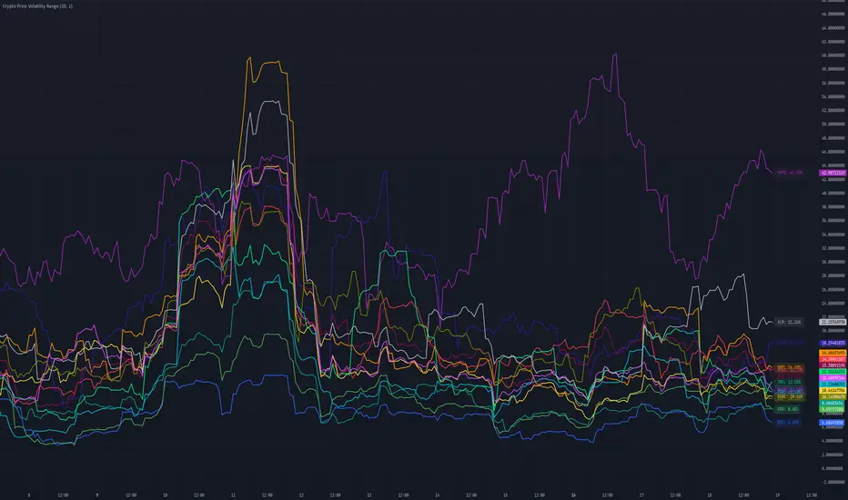
Crypto Price Volatility Range# Cryptocurrency Price Volatility Range Indicator
This TradingView indicator is a visualization tool for tracking historical volatility across multiple major cryptocurrencies.
## Features
- Real-time volatility tracking for 14 major cryptocurrencies
- Customizable period and standard deviation multiplier
- Individual color coding for each currency pair
- Optional labels showing current volatility values in percentage
## Supported Cryptocurrencies
- Bitcoin (BTC)
- Ethereum (ETH)
- Avalanche (AVAX)
- Dogecoin (DOGE)
- Hype (HYPE)
- Ripple (XRP)
- Binance Coin (BNB)
- Cardano (ADA)
- Tron (TRX)
- Chainlink (LINK)
- Shiba Inu (SHIB)
- Toncoin (TON)
- Sui (SUI)
- Stellar (XLM)
## Settings
- **Period**: Timeframe for volatility calculation (default: 20)
- **Standard Deviation Multiplier**: Multiplier for standard deviation (default: 1.0)
- **Show Labels**: Toggle label display on/off
## Calculation Method
The indicator calculates volatility using the following method:
1. Calculate daily logarithmic returns
2. Compute standard deviation over the specified period
3. Annualize (multiply by √252)
4. Convert to percentage (×100)
## Usage
1. Add the indicator to your TradingView chart
2. Adjust parameters as needed
3. Monitor volatility lines for each cryptocurrency
4. Enable labels to see precise current volatility values
## Notes
- This indicator displays in a separate window, not as an overlay
- Volatility values are annualized
- Data for each currency pair is sourced from USD pairs
Ultimate Volatility RateUltimate Volatility Rate
This indicator measures the volatility of price movements.
Support and Resistance Identification:
High volatility periods indicate larger price movements, which can be useful in assessing the potential for support and resistance levels to be broken.
Stop Loss (SL) and Take Profit (TP) Calculations:
The average volatility can be used to calculate dynamic Stop Loss (SL) and Take Profit (TP) levels:
SL: Placing it at a certain volatility multiplier below/above the entry price.
TP: Setting it at a certain volatility multiplier below/above the entry price.
For example:
SL: Entry price +/- (UVR × 1.5)
TP: Entry price +/- (UVR × 2)
Market Condition Analysis:
When the indicator value is high, it suggests that the market is volatile (active).
When the value is low, it indicates the market is in consolidation (sideways movement).
This information helps traders decide whether to take trend-following or consolidation-based positions.
Trend Reversal Monitoring:
A sudden increase in volatility often signals the start of a strong trend.
Conversely, a decrease in volatility can signal the slowing down or end of a trend.

Conditional Volatility Explosion/ContractionThis indicator identifies zones of potential volatility expansion by analyzing the contraction and expansion of volatility bands, which are conditioned by the relationship of the price to moving averages
Volatility Squeeze: When the bands contract, it indicates a potential buildup in market tension, often preceding a significant price movement.
Volatility Expansion: When the bands expand, it signals the release of built-up tension, often resulting in increased volatility.
Trend Confirmation: The bands are active only when the price aligns with the moving average condition, helping to filter out less relevant signals during non-trending markets.
Upper Band: Displays as a red band when the volatility condition is met.
Represents the upper boundary of potential price action during high volatility.
Lower Band: Displays as a green band when the volatility condition is met.
Represents the lower boundary of potential price action during high volatility.
Fill Areas: The areas between the EMA and the bands are filled with transparent colors:
Red for the upper fill.
Green for the lower fill.
These highlights help visualize zones of potential volatility explosion.

Bayesian Price Projection Model [Pinescriptlabs]📊 Dynamic Price Projection Algorithm 📈
This algorithm combines **statistical calculations**, **technical analysis**, and **Bayesian theory** to forecast a future price while providing **uncertainty ranges** that represent upper and lower bounds. The calculations are designed to adjust projections by considering market **trends**, **volatility**, and the historical probabilities of reaching new highs or lows.
Here’s how it works:
🚀 Future Price Projection
A dynamic calculation estimates the future price based on three key elements:
1. **Trend**: Defines whether the market is predisposed to move up or down.
2. **Volatility**: Quantifies the magnitude of the expected change based on historical fluctuations.
3. **Time Factor**: Uses the logarithm of the projected period (`proyeccion_dias`) to adjust how time impacts the estimate.
🧠 **Bayesian Probabilistic Adjustment**
- Conditional probabilities are calculated using **Bayes' formula**:
\
This models future events using conditional information:
- **Probability of reaching a new all-time high** if the price is trending upward.
- **Probability of reaching a new all-time low** if the price is trending downward.
- These probabilities refine the future price estimate by considering:
- **Higher volatility** increases the likelihood of hitting extreme levels (highs/lows).
- **Market trends** influence the expected price movement direction.
🌟 **Volatility Calculation**
- Volatility is measured using the **ATR (Average True Range)** indicator with a 14-period window. This reflects the average amplitude of price fluctuations.
- To express volatility as a percentage, the ATR is normalized by dividing it by the closing price and multiplying it by 200.
- Volatility is then categorized into descriptive levels (e.g., **Very Low**, **Low**, **Moderate**, etc.) for better interpretation.
---
🎯 **Deviation Limits (Upper and Lower)**
- The upper and lower limits form a **projected range** around the estimated future price, providing a framework for uncertainty.
- These limits are calculated by adjusting the ATR using:
- A user-defined **multiplier** (`factor_desviacion`).
- **Bayesian probabilities** calculated earlier.
- The **square root of the projected period** (`proyeccion_dias`), incorporating the principle that uncertainty grows over time.
🔍 **Interpreting the Model**
This can be seen as a **dynamic probabilistic model** that:
- Combines **technical analysis** (trends and ATR).
- Refines probabilities using **Bayesian theory**.
- Provides a **visual projection range** to help you understand potential future price movements and associated uncertainties.
⚡ Whether you're analyzing **volatile markets** or confirming **bullish/bearish scenarios**, this tool equips you with a robust, data-driven approach! 🚀
Español :
📊 Algoritmo de Proyección de Precio Dinámico 📈
Este algoritmo combina **cálculos estadísticos**, **análisis técnico** y **la teoría de Bayes** para proyectar un precio futuro, junto con rangos de **incertidumbre** que representan los límites superior e inferior. Los cálculos están diseñados para ajustar las proyecciones considerando la **tendencia del mercado**, **volatilidad** y las probabilidades históricas de alcanzar nuevos máximos o mínimos.
Aquí se explica su funcionamiento:
🚀 **Proyección de Precio Futuro**
Se realiza un cálculo dinámico del precio futuro estimado basado en tres elementos clave:
1. **Tendencia**: Define si el mercado tiene predisposición a subir o bajar.
2. **Volatilidad**: Determina la magnitud del cambio esperado en función de las fluctuaciones históricas.
3. **Factor de Tiempo**: Usa el logaritmo del período proyectado (`proyeccion_dias`) para ajustar cómo el tiempo afecta la estimación.
🧠 **Ajuste Probabilístico con la Teoría de Bayes**
- Se calculan probabilidades condicionales mediante la fórmula de **Bayes**:
\
Esto permite modelar eventos futuros considerando información condicional:
- **Probabilidad de alcanzar un nuevo máximo histórico** si el precio sube.
- **Probabilidad de alcanzar un nuevo mínimo histórico** si el precio baja.
- Estas probabilidades ajustan la estimación del precio futuro considerando:
- **Mayor volatilidad** aumenta la probabilidad de alcanzar niveles extremos (máximos/mínimos).
- **La tendencia del mercado** afecta la dirección esperada del movimiento del precio.
🌟 **Cálculo de Volatilidad**
- La volatilidad se mide usando el indicador **ATR (Average True Range)** con un período de 14 velas. Este indicador refleja la amplitud promedio de las fluctuaciones del precio.
- Para obtener un valor porcentual, el ATR se normaliza dividiéndolo por el precio de cierre y multiplicándolo por 200.
- Además, se clasifica esta volatilidad en categorías descriptivas (e.g., **Muy Baja**, **Baja**, **Moderada**, etc.) para facilitar su interpretación.
🎯 **Límites de Desviación (Superior e Inferior)**
- Los límites superior e inferior representan un **rango proyectado** en torno al precio futuro estimado, proporcionando un marco para la incertidumbre.
- Estos límites se calculan ajustando el ATR según:
- Un **multiplicador** definido por el usuario (`factor_desviacion`).
- Las **probabilidades condicionales** calculadas previamente.
- La **raíz cuadrada del período proyectado** (`proyeccion_dias`), lo que incorpora el principio de que la incertidumbre aumenta con el tiempo.
---
🔍 **Interpretación del Modelo**
Este modelo se puede interpretar como un **modelo probabilístico dinámico** que:
- Integra **análisis técnico** (tendencias y ATR).
- Ajusta probabilidades utilizando **la teoría de Bayes**.
- Proporciona un **rango de proyección visual** para ayudarte a entender los posibles movimientos futuros del precio y su incertidumbre.
⚡ Ya sea que estés analizando **mercados volátiles** o confirmando **escenarios alcistas/bajistas**, ¡esta herramienta te ofrece un enfoque robusto y basado en datos! 🚀

Same Day Price Volatility [5ema]Indicator visualizes the price volatility of the current day alongside historical volatility patterns of the same weekday across previous weeks. It highlights high, low, and total volatility ranges with interactive boxes, labels, and average lines for easy analysis.
=====
A. How to Calculate?
*Current Day Volatility:
High Volatility: High − Open
Low Volatility: Low − Open
Total Volatility: High − Low
*Historical Volatility:
The script scans historical data for the same weekday over the past number weeks (default: 12 weeks).
It calculates the high, low, and total volatility for each historical same day.
Average Lines:
Averages for high, low, and total volatility are calculated from historical values and plotted as dotted lines.
=====
B. How to Set Up?
Inputs:
Weeks Back (nb): Number of past weeks to include in historical calculations (default: 12).
Position (pos): Horizontal offset for displaying boxes and labels (default: 50).
Colors: Customize box colors for high, low, and total volatility ranges.
=====
C. How to Use?
Analyze Current Day Volatility:
The script displays boxes for today's high, low, and total volatility relative to the opening price.
Labels provide detailed tooltips for easy interpretation.
Compare Historical Patterns:
Historical volatility boxes for the same weekday are plotted for up to number weeks.
Labels display the exact date and volatility values for each historical day.
Utilize Average Volatility Lines:
Use the average lines to compare today's performance against historical averages for high, low, and total volatility.
Customizing Visualization:
Adjust the pos input to reposition the boxes and labels if overlapping with price data.
Modify the colors to suit your preferred visual style.
=====
This indicator is for reference only, you need your own method and strategy.
If you have any questions, please let me know in the comments.

Volatility % (Standard Deviation of Returns)This script takes closing prices of candles to measure the Standard Deviation (σ) which is then used to calculate the volatility by taking the stdev of the last 30 candles and multiplying it by the root of the trading days in a year, month and week. It then multiplies that number by 100 to show a percentage.
Default settings are annual volatility (252 candles, red), monthly volatility (30 candles, blue) and weekly volatility (5 candles, green) if you use daily candles. It is open source so you can increase the number of candles with which the stdev is calculated, and change the number of the root that multiplies the stdev.

Z Value AlertZ Value Alert analyzes daily price movements by evaluating fluctuations relative to historical volatility. It calculates the daily percentage change in the closing price, the average of this change over 252 days, and the standard deviation. Using these values, a Z-Score is calculated, indicating how much the current price change deviates from the historical range of fluctuations.
The user can set a threshold in standard deviations (Z-Score). When the absolute Z-Score exceeds this threshold, a significant movement is detected, indicating increased volatility. The Z-Score is visualized as a histogram, and an alert can be triggered when a significant movement occurs.
The number of trading days used to calculate historical volatility is adjustable, allowing the Sigma Move Alert to be tailored to various trading strategies and analysis periods.
Additionally, a dropdown option for the calculation method is available in the input menu, allowing the user to select between:
Normal: Calculates the percentage change in closing prices without using the logarithm.
Logarithmic: Uses the natural logarithm of daily returns. This method is particularly suitable for longer timeframes and scientific analyses, as logarithmic returns are additive.
These comprehensive features allow for precise customization of the Sigma Move Alert to individual needs and specific market conditions.

DIVERGENCE SPOT X P.FUTURES (INVERTED VERSION) [GUSLM]Many asked me to change the positive position x negative(of "DIVERGENCE SPOT X P.FUTURES"). being maybe no intuitive for some coins and situations....
So, Now on this version you are going to have UP moves for Upwards from derivatives ( p. Futures with Higher prices than Spot prices), and Dowwards for Negative Futures derivatives. ( it will match the future funding rates probably)
The "pushs" now are in the oposite direction.
Look at the DIVERGENCE SPOT X P.FUTURES script for a better view about it.
For instance:
This version is better for normal coin and market - where the derivatives go in the direction of the price and the coin will have a positive FR(funding) when going up, and maybe sometimes negatives when going down.
The First non inverted version: is better for manipulated coins, where you have pushs and pulls, to try to build a negative funding while hold longs positions. it will go up with negative FR. - Shorters paying the longs and being liquidated in the way..
But you can chose one and adaptd to use only one fot both situations, only need to take a look on the market and define whats going on with the books and prices moves.

30D Vs 90D Historical VolatilityVolatility equals risk for an underlying asset's price meaning bullish volatility is bearish for prices while bearish volatility is bullish. This compares 30-Day Historical Volatility to 90-Day Historical Volatility.
When the 30-Day crosses under the 90-day, this is typically when asset prices enter a bullish trend.
Conversely, When the 30-Day crosses above the 90-Day, this is when asset prices enter a bearish trend.
Peaks in volatility are bullish divergences while troughs are bearish divergences.

Relative VolatilityRelative Volatility is a technical indicator designed to assess changes in market volatility by comparing fast and slow Average True Range (ATR) values. It operates by subtracting a slower ATR (e.g., 50-period ATR) from a faster ATR (e.g., 20-period ATR) and visualizing the result as a histogram. This enables traders to determine whether volatility is increasing or decreasing over time.
This indicator can help traders recognize volatility trends, which can inform decisions related to trade entries, exits, and risk management.
Interpreting Volatility Changes
Increasing Volatility: When the histogram is above zero, it indicates that the fast ATR is greater than the slow ATR, signifying an increase in short-term volatility compared to the long-term average. This may suggest heightened market activity and potential trading opportunities.
Decreasing Volatility: When the histogram is below zero, it shows that the fast ATR is less than the slow ATR, indicating a decrease in short-term volatility relative to the long-term average. This may suggest consolidating markets or reduced trading activity.
Relative Volatility assists traders in monitoring and analyzing changes in market volatility, providing insights that can enhance trading strategies and decision-making processes.

Crypto Volatility Bitcoin Correlation Strategy Description:
The Crypto Volatility Bitcoin Correlation Strategy is designed to leverage market volatility specifically in Bitcoin (BTC) using a combination of volatility indicators and trend-following techniques. This strategy utilizes the VIXFix (a volatility indicator adapted for crypto markets) and the BVOL7D (Bitcoin 7-Day Volatility Index from BitMEX) to identify periods of high volatility, while confirming trends with the Exponential Moving Average (EMA). These components work together to offer a comprehensive system that traders can use to enter positions when volatility and trends are aligned in their favor.
Key Features:
VIXFix (Volatility Index for Crypto Markets): This indicator measures the highest price of Bitcoin over a set period and compares it with the current low price to gauge market volatility. A rise in VIXFix indicates increasing market volatility, signaling that large price movements could occur.
BVOL7D (Bitcoin 7-Day Volatility Index): This volatility index, provided by BitMEX, measures the volatility of Bitcoin over the past 7 days. It helps traders monitor the recent volatility trend in the market, particularly useful when making short-term trading decisions.
Exponential Moving Average (EMA): The 50-period EMA acts as a trend indicator. When the price is above the EMA, it suggests the market is in an uptrend, and when the price is below the EMA, it suggests a downtrend.
How It Works:
Long Entry: A long position is triggered when both the VIXFix and BVOL7D indicators are rising, signaling increased volatility, and the price is above the 50-period EMA, confirming that the market is trending upward.
Exit: The strategy exits the position when the price crosses below the 50-period EMA, which signals a potential weakening of the uptrend and a decrease in volatility.
This strategy ensures that traders only enter positions when the volatility aligns with a clear trend, minimizing the risk of entering trades during periods of market uncertainty.
Testing and Timeframe:
This strategy has been tested on Bitcoin using the daily timeframe, which provides a longer-term perspective on market trends and volatility. However, users can adjust the timeframe according to their trading preferences. It is crucial to note that this strategy does not include comprehensive risk management, aside from the exit condition when the price crosses below the EMA. Users are strongly advised to implement their own risk management techniques, such as setting appropriate stop-loss levels, to safeguard their positions during high volatility periods.
Utility:
The Crypto Volatility Bitcoin Correlation Strategy is particularly well-suited for traders who aim to capitalize on the high volatility often seen in the Bitcoin market. By combining volatility measurements (VIXFix and BVOL7D) with a trend-following mechanism (EMA), this strategy helps identify optimal moments for entering and exiting trades. This approach ensures that traders participate in potentially profitable market moves while minimizing exposure during times of uncertainty.
Use Cases:
Volatility-Based Entries: Traders looking to take advantage of market volatility spikes will find this strategy useful for timing entry points during market swings.
Trend Confirmation: By using the EMA as a confirmation tool, traders can avoid entering trades that go against the trend, which can result in significant losses during volatile market conditions.
Risk Management: While the strategy exits when price falls below the EMA, it is important to recognize that this is not a full risk management system. Traders should use caution and integrate additional risk measures, such as stop-losses and position sizing, to better manage potential losses.
How to Use:
Step 1: Monitor the VIXFix and BVOL7D indicators. When both are rising and the Bitcoin price is above the EMA, the strategy will trigger a long entry, indicating that the market is experiencing increased volatility with a confirmed uptrend.
Step 2: Exit the position when the price drops below the 50-period EMA, signaling that the trend may be reversing or weakening, reducing the likelihood of continued upward price movement.
This strategy is open-source and is intended to help traders navigate volatile market conditions, particularly in Bitcoin, using proven indicators for volatility and trend confirmation.
Risk Disclaimer:
This strategy has been tested on the daily timeframe of Bitcoin, but users should be aware that it does not include built-in risk management except for the below-EMA exit condition. Users should be extremely cautious when using this strategy and are encouraged to implement their own risk management, such as using stop-losses, position sizing, and setting appropriate limits. Trading involves significant risk, and this strategy does not guarantee profits or prevent losses. Past performance is not indicative of future results. Always test any strategy in a demo environment before applying it to live markets.

Probability GoldThis is a leading indicator designed for the 1 minute chart, and while it works on any time frame, I haven't tested it's practicality outside of the 1 minute chart. This uses historical data and applies statistical analysis to key metrics of momentum. The data is filtered by "time of day" as well as "day of week", but be mindful that the "day of week" option reduces your total amount of data points, and will not work well on new stocks. This indicator also uses binary/gaussian distribution concepts to create channels and pockets which act as seemingly magnetic forces. This is all speculative. Do not use this indicator on its own. This is intended to do nothing more than to show you whether if, on average, the historical data under the same time and rate of change conditions, goes for or against your trade. Use it in conjunction with your most trusted and classic indicators. This can act as a small nudge, letting you now the chances of what you have already established in your mind. This is HIGHLY experimental, made by an amateur, and also very pretty. So, enjoy!

Standard Deviation based Upper Lower RangeThis script makes use of historical data for finding the standard deviation on daily returns. Based on the mean and standard deviation, the upper and lower range for the stock is shown upto 2x standard deviation. These bounds can be treated as volatility range for the next n trading sessions. This volatility is based on historical data. Users can change the lookback historical period, and can also set the time period (days) for upcoming trading sessions.
This indicator can be useful in determining stoploss and target levels along with the traditional support/resistance levels. It can also be useful in option trading where one needs to determine a range beyond which it is safe to sell an option.
A range of 1 SD has around 65% to 68% probability that it will not be breached. A range of 2 SD has around 95% probability that it will not be breached.
The indicator is based on Normal distribution theory. In future editions, I envision to also calculate the skewness and kurtosis so that we can determine if a stock is properly following Normal Distribution theory. That may further favor the calculated range.

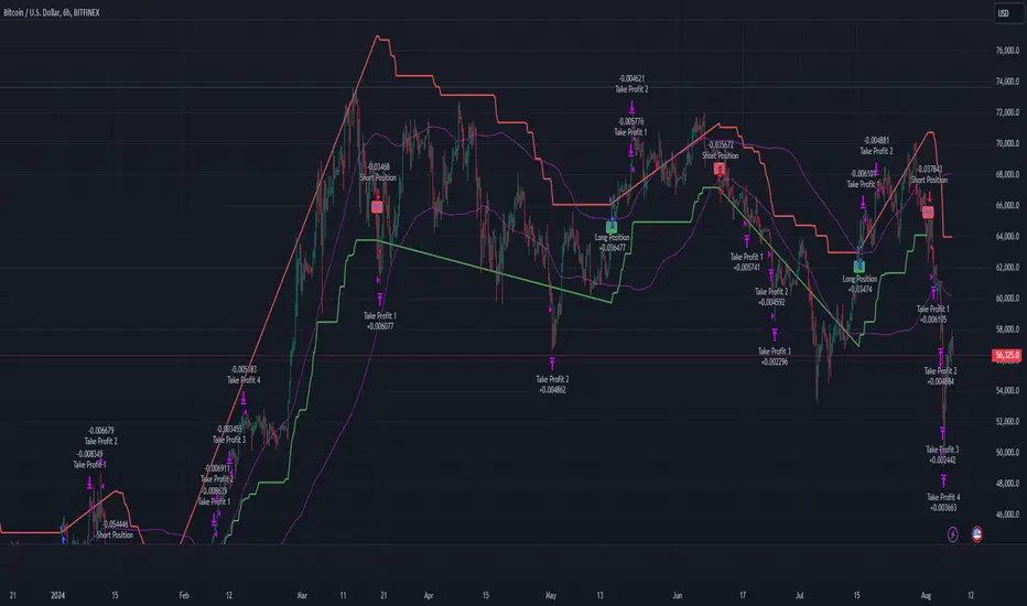
Multi-Step Vegas SuperTrend - strategy [presentTrading]Long time no see! I am back : ) Please allow me to gain some warm-up.
█ Introduction and How it is Different
The "Vegas SuperTrend Strategy" is an enhanced trading strategy that leverages both the Vegas Channel and SuperTrend indicators to generate buy and sell signals.
What sets this strategy apart from others is its dynamic adjustment to market volatility and its multi-step take profit mechanism. Unlike traditional single-step profit-taking approaches, this strategy allows traders to systematically scale out of positions at predefined profit levels, thereby optimizing their risk-reward ratio and maximizing potential gains.
BTCUSD 6hr performance
█ Strategy, How it Works: Detailed Explanation
The Vegas SuperTrend Strategy combines the strengths of the Vegas Channel and SuperTrend indicators to identify market trends and generate trade signals. The following subsections delve into the details of how each component works and how they are integrated.
🔶 Vegas Channel Calculation
The Vegas Channel is based on a simple moving average (SMA) and the standard deviation (STD) of the closing prices over a specified period. The channel is defined by upper and lower bounds that are dynamically adjusted based on market volatility.
Simple Moving Average (SMA):
SMA_vegas = (1/N) * Σ(Close_i) for i = 0 to N-1
where N is the length of the Vegas Window.
Standard Deviation (STD):
STD_vegas = sqrt((1/N) * Σ(Close_i - SMA_vegas)^2) for i = 0 to N-1
Vegas Channel Upper and Lower Bounds:
VegasChannelUpper = SMA_vegas + STD_vegas
VegasChannelLower = SMA_vegas - STD_vegas
The details are here:
🔶 Trend Detection and Trade Signals
The strategy determines the current market trend based on the closing price relative to the SuperTrend bounds:
Market Trend:
MarketTrend = 1 if Close > SuperTrendPrevLower
-1 if Close < SuperTrendPrevUpper
Previous Trend otherwise
Trade signals are generated when there is a shift in the market trend:
Bullish Signal: When the market trend shifts from -1 to 1.
Bearish Signal: When the market trend shifts from 1 to -1.
🔶 Multi-Step Take Profit Mechanism
The strategy incorporates a multi-step take profit mechanism that allows for partial exits at predefined profit levels. This helps in locking in profits gradually and reducing exposure to market reversals.
Take Profit Levels:
The take profit levels are calculated as percentages of the entry price:
TakeProfitLevel_i = EntryPrice * (1 + TakeProfitPercent_i/100) for long positions
TakeProfitLevel_i = EntryPrice * (1 - TakeProfitPercent_i/100) for short positions
Multi-steps take profit local picture:
█ Trade Direction
The trade direction can be customized based on the user's preference:
Long: The strategy only takes long positions.
Short: The strategy only takes short positions.
Both: The strategy can take both long and short positions based on the market trend.
█ Usage
To use the Vegas SuperTrend Strategy, follow these steps:
Configure Input Settings:
- Set the ATR period, Vegas Window length, SuperTrend Multiplier, and Volatility Adjustment Factor.
- Choose the desired trade direction (Long, Short, Both).
- Enable or disable the take profit mechanism and set the take profit percentages and amounts for each step.
█ Default Settings
The default settings of the strategy are designed to provide a balanced approach to trading. Below is an explanation of each setting and its effect on the strategy's performance:
ATR Period (10): This setting determines the length of the ATR used in the SuperTrend calculation. A longer period smoothens the ATR, making the SuperTrend less sensitive to short-term volatility. A shorter period makes the SuperTrend more responsive to recent price movements.
Vegas Window Length (100): This setting defines the period for the Vegas Channel's moving average. A longer window provides a broader view of the market trend, while a shorter window makes the channel more responsive to recent price changes.
SuperTrend Multiplier (5): This base multiplier adjusts the sensitivity of the SuperTrend to the ATR. A higher multiplier makes the SuperTrend less sensitive, reducing the frequency of trade signals. A lower multiplier increases sensitivity, generating more signals.
Volatility Adjustment Factor (5): This factor dynamically adjusts the SuperTrend multiplier based on the width of the Vegas Channel. A higher factor increases the sensitivity of the SuperTrend to changes in market volatility, while a lower factor reduces it.
Take Profit Percentages (3.0%, 6.0%, 12.0%, 21.0%): These settings define the profit levels at which portions of the trade are exited. They help in locking in profits progressively as the trade moves in favor.
Take Profit Amounts (25%, 20%, 10%, 15%): These settings determine the percentage of the position to exit at each take profit level. They are distributed to ensure that significant portions of the trade are closed as the price reaches the set levels, reducing exposure to reversals.
Adjusting these settings can significantly impact the strategy's performance. For instance, increasing the ATR period or the SuperTrend multiplier can reduce the number of trades, potentially improving the win rate but also missing out on some profitable opportunities. Conversely, lowering these values can increase trade frequency, capturing more short-term movements but also increasing the risk of false signals.
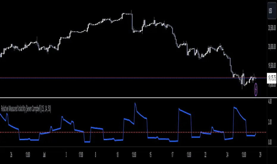
Relative Measured Volatility [Seven Campbell]Relative Measured Volatility
Overview:
This indicator measures the current daily volatility of an asset and compares it to the average volatility observed over the past 15 days. It provides a dynamic gauge of how much the market’s volatility is deviating from its recent historical norms.
Key Features:
Dynamic Comparison: The indicator calculates the standard deviation of daily price changes over a user-defined period (default is 14 days) and compares it to a smoothed average of this volatility over the last 15 days. This creates a "moving measuring stick" to highlight periods of unusually high or low volatility.
Customizable Settings:
Lookback Period: Set to 15 days by default, this period defines the historical window used to calculate the average volatility.
Volatility Length: Adjustable length (default is 14) for the standard deviation calculation, allowing you to fine-tune the sensitivity of the volatility measurement.
Smoothing Length: Set to 50 by default, this parameter smooths the volatility data to highlight longer-term trends.
How It Works:
Volatility Calculation: The indicator computes the daily returns using the logarithmic change in closing prices. It then calculates the standard deviation of these returns over the specified volatility length.
Smoothing: The standard deviation values are smoothed using a simple moving average over the smoothing length, providing a clearer view of trends.
Relative Measurement: The current daily volatility is divided by the smoothed volatility, giving a relative value. A value above 1 indicates higher volatility than the average over the past 15 days, while a value below 1 suggests lower volatility.
Visual Representation:
Line Plot: The relative volatility is plotted as a line, allowing you to quickly see changes in volatility relative to the historical average.
Reference Line: A horizontal line at 1 is included for easy reference. Values above this line indicate periods of higher-than-average volatility, and values below suggest lower-than-average volatility.
Use Cases:
Market Sentiment Analysis: Identify periods of high or low volatility to gauge market sentiment.
Trade Timing: Use the indicator to decide on entry and exit points, especially in volatile or calm market conditions.
Risk Management: Monitor volatility to adjust position sizes and stop-loss levels dynamically.
Example Usage:
When the line rises above 1, it signals increasing volatility, which may be a good time to take profit or adjust your stop-loss orders.
When the line drops below 1, it indicates lower volatility, potentially highlighting a stable market period.
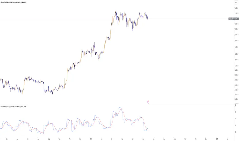
Historical Volatility (adjustable time period)Historical Volatility with Adjustable Time Period and Moving Average
This indicator calculates the historical volatility of an asset within a user-defined date range. Volatility is a measure of the dispersion of returns and is commonly used to assess the risk and potential price fluctuations of an asset.
How It Works
User-Defined Date Range: You can specify the start and end dates to focus on a particular period for volatility calculation. This is useful for analyzing specific historical events or trends within a defined timeframe.
Daily Returns Calculation: The script calculates the daily returns as the percentage change between the current close price and the previous close price. This percentage change is essential for determining the asset's volatility.
Volatility Calculation: The historical volatility is computed as the standard deviation of the daily returns over a specified period. The standard deviation is a statistical measure that quantifies the amount of variation or dispersion in a set of values.
Moving Average: An optional feature allows you to plot a moving average of the volatility. You can customize the type (SMA, EMA, WMA, VWMA) and the period of the moving average, helping to smooth out the volatility data and identify trends.
Indicator Settings
Start Date: Select the beginning date of the period for which you want to calculate volatility.
End Date: Select the end date of the period.
Period: Set the number of bars (days) over which to calculate the average volatility.
Show Moving Average: Toggle to display the moving average of the volatility.
Moving Average Period: Define the length of the moving average.
Moving Average Type: Choose the type of moving average: Simple (SMA), Exponential (EMA), Weighted (WMA), or Volume-Weighted (VWMA).
How to Use
Configure Date Range: Set the start and end dates to focus on the specific historical period you are interested in.
Adjust Period for Volatility Calculation: Select the period over which you want to calculate the average volatility. A shorter period will be more sensitive to recent price changes, while a longer period will provide a more smoothed view.
Enable and Configure Moving Average: If desired, enable the moving average and select the type and period that best fits your analysis style.
Example Use Cases
Market Analysis: Identify periods of high or low volatility to assess market conditions.
Risk Management: Use historical volatility to evaluate the risk associated with a particular asset.
Event Impact: Analyze how specific events within the selected date range affected the asset's volatility.
By providing these functionalities, this indicator is a valuable tool for traders looking to understand and analyze the volatility of assets over custom time periods with the flexibility of adding a moving average for trend analysis.
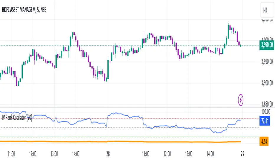
IV Rank Oscillator by dinvestorqShort Title: IVR OscSlg
Description:
The IV Rank Oscillator is a custom indicator designed to measure and visualize the Implied Volatility (IV) Rank using Historical Volatility (HV) as a proxy. This indicator helps traders determine whether the current volatility level is relatively high or low compared to its historical levels over a specified period.
Key Features :
Historical Volatility (HV) Calculation: Computes the historical volatility based on the standard deviation of logarithmic returns over a user-defined period.
IV Rank Calculation: Normalizes the current HV within the range of the highest and lowest HV values over the past 252 periods (approximately one year) to generate the IV Rank.
IV Rank Visualization: Plots the IV Rank, along with reference lines at 50 (midline), 80 (overbought), and 20 (oversold), making it easy to interpret the relative volatility levels.
Historical Volatility Plot: Optionally plots the Historical Volatility for additional reference.
Usage:
IV Rank : Use the IV Rank to assess the relative level of volatility. High IV Rank values (close to 100) indicate that the current volatility is high relative to its historical range, while low IV Rank values (close to 0) indicate low relative volatility.
Reference Lines: The overbought (80) and oversold (20) lines help identify extreme volatility conditions, aiding in trading decisions.
Example Use Case:
A trader can use the IV Rank Oscillator to identify potential entry and exit points based on the volatility conditions. For instance, a high IV Rank may suggest a period of high market uncertainty, which could be a signal for options traders to consider strategies like selling premium. Conversely, a low IV Rank might indicate a more stable market condition.
Parameters:
HV Calculation Length: Adjustable period length for the historical volatility calculation (default: 20 periods).
This indicator is a powerful tool for options traders, volatility analysts, and any market participant looking to gauge market conditions based on historical volatility patterns.
FOMO Alert (Miu)This indicator won't plot anything to the chart.
Please follow steps below to set your alarms based on price range variation:
1) Add indicator to the chart
2) Go to settings
3) Choose timeframe which will be used to calculate bars
4) Choose how many bars which will be used to calculate max and min range
5) Choose max and min range variation (%) to trigger alerts
5) Choose up to 6 different symbols to get alert notification
6) Once all is set go back to the chart and click on 3 dots to set alert in this indicator, rename your alert and confirm
7) You can remove indicator after alert is set and it'll keep working as expected
What does this indicator do?
This indicator will generate alerts based on following conditions:
- If min and max prices reach the range (%) from amount of bars on timeframe set for any symbol checked it will trigger an alert.
- If next set of bars reaches higher range than before it will trigger an alert with new data
- If next set of bars doesn't reach higher range than before it will not trigger alerts, even if they are above the range set (this is to prevent the alert to keep triggering with high frequency)
Once condition is met it will send an alert with the following information:
- Symbol name (e.g: BTC, ETH, LTC)
- Range achieved (e.g: 3,03%)
- Current symbol price and current bar direction (e.g: 63,477.1 ▲)
This script will request lowest and highest prices through request.security() built-in function from all different symbols within the range set. It also requests symbols' price (close) and amount of digits (mintick) for each symbol to send alerts with correct value.
This script was developed with main purpose to send alerts when there are strong price movements and I decided to share with community so anyone can set different parameters for different purposes.
Feel free to give feedbacks on comments section below.
Enjoy!
