S&P500 Net Issues Block 10Description:
This indicator calculates and plots net advancers minus decliners for 13 predefined blocks of S&P 500 stocks. Each block represents a sector or a selected subset of stocks.
Features:
Shows net issues (advancers – decliners) for each block separately.
13 blocks plotted with distinct colors for easy identification.
Fully compatible with 1-minute, intraday, or higher timeframe charts.
Ideal for identifying sector momentum and market breadth trends.
Can be used standalone or combined with other indicators such as market indices (e.g., S&P 500 futures or TICK).
Usage:
Green/red/blue/orange lines represent different blocks; positive values indicate more advancing stocks than declining, negative values indicate more declining stocks.
Best viewed on intraday charts for short-term market breadth analysis.
Disclaimer:
This indicator is for educational and analytical purposes only. Not a buy/sell signal. Use proper risk management and verify data before trading.
Tìm kiếm tập lệnh với "标普500+指数+构成"

S&P500 Net Issues Block 9Description:
This indicator calculates and plots net advancers minus decliners for 13 predefined blocks of S&P 500 stocks. Each block represents a sector or a selected subset of stocks.
Features:
Shows net issues (advancers – decliners) for each block separately.
13 blocks plotted with distinct colors for easy identification.
Fully compatible with 1-minute, intraday, or higher timeframe charts.
Ideal for identifying sector momentum and market breadth trends.
Can be used standalone or combined with other indicators such as market indices (e.g., S&P 500 futures or TICK).
Usage:
Green/red/blue/orange lines represent different blocks; positive values indicate more advancing stocks than declining, negative values indicate more declining stocks.
Best viewed on intraday charts for short-term market breadth analysis.
Disclaimer:
This indicator is for educational and analytical purposes only. Not a buy/sell signal. Use proper risk management and verify data before trading.

S&P500 Net Issues Block 8Description:
This indicator calculates and plots net advancers minus decliners for 13 predefined blocks of S&P 500 stocks. Each block represents a sector or a selected subset of stocks.
Features:
Shows net issues (advancers – decliners) for each block separately.
13 blocks plotted with distinct colors for easy identification.
Fully compatible with 1-minute, intraday, or higher timeframe charts.
Ideal for identifying sector momentum and market breadth trends.
Can be used standalone or combined with other indicators such as market indices (e.g., S&P 500 futures or TICK).
Usage:
Green/red/blue/orange lines represent different blocks; positive values indicate more advancing stocks than declining, negative values indicate more declining stocks.
Best viewed on intraday charts for short-term market breadth analysis.
Disclaimer:
This indicator is for educational and analytical purposes only. Not a buy/sell signal. Use proper risk management and verify data before trading.

S&P500 Net Issues Block 7Description:
This indicator calculates and plots net advancers minus decliners for 13 predefined blocks of S&P 500 stocks. Each block represents a sector or a selected subset of stocks.
Features:
Shows net issues (advancers – decliners) for each block separately.
13 blocks plotted with distinct colors for easy identification.
Fully compatible with 1-minute, intraday, or higher timeframe charts.
Ideal for identifying sector momentum and market breadth trends.
Can be used standalone or combined with other indicators such as market indices (e.g., S&P 500 futures or TICK).
Usage:
Green/red/blue/orange lines represent different blocks; positive values indicate more advancing stocks than declining, negative values indicate more declining stocks.
Best viewed on intraday charts for short-term market breadth analysis.
Disclaimer:
This indicator is for educational and analytical purposes only. Not a buy/sell signal. Use proper risk management and verify data before trading.

S&P500 Net Issues Block 6Description:
This indicator calculates and plots net advancers minus decliners for 13 predefined blocks of S&P 500 stocks. Each block represents a sector or a selected subset of stocks.
Features:
Shows net issues (advancers – decliners) for each block separately.
13 blocks plotted with distinct colors for easy identification.
Fully compatible with 1-minute, intraday, or higher timeframe charts.
Ideal for identifying sector momentum and market breadth trends.
Can be used standalone or combined with other indicators such as market indices (e.g., S&P 500 futures or TICK).
Usage:
Green/red/blue/orange lines represent different blocks; positive values indicate more advancing stocks than declining, negative values indicate more declining stocks.
Best viewed on intraday charts for short-term market breadth analysis.
Disclaimer:
This indicator is for educational and analytical purposes only. Not a buy/sell signal. Use proper risk management and verify data before trading.

S&P500 Net Issues - Block 5Description:
This indicator calculates and plots net advancers minus decliners for 13 predefined blocks of S&P 500 stocks. Each block represents a sector or a selected subset of stocks.
Features:
Shows net issues (advancers – decliners) for each block separately.
13 blocks plotted with distinct colors for easy identification.
Fully compatible with 1-minute, intraday, or higher timeframe charts.
Ideal for identifying sector momentum and market breadth trends.
Can be used standalone or combined with other indicators such as market indices (e.g., S&P 500 futures or TICK).
Usage:
Green/red/blue/orange lines represent different blocks; positive values indicate more advancing stocks than declining, negative values indicate more declining stocks.
Best viewed on intraday charts for short-term market breadth analysis.
Disclaimer:
This indicator is for educational and analytical purposes only. Not a buy/sell signal. Use proper risk management and verify data before trading.

S&P500 Net Issues Block 3Description:
This indicator calculates and plots net advancers minus decliners for 13 predefined blocks of S&P 500 stocks. Each block represents a sector or a selected subset of stocks.
Features:
Shows net issues (advancers – decliners) for each block separately.
13 blocks plotted with distinct colors for easy identification.
Fully compatible with 1-minute, intraday, or higher timeframe charts.
Ideal for identifying sector momentum and market breadth trends.
Can be used standalone or combined with other indicators such as market indices (e.g., S&P 500 futures or TICK).
Usage:
Green/red/blue/orange lines represent different blocks; positive values indicate more advancing stocks than declining, negative values indicate more declining stocks.
Best viewed on intraday charts for short-term market breadth analysis.
Disclaimer:
This indicator is for educational and analytical purposes only. Not a buy/sell signal. Use proper risk management and verify data before trading.

S&P500 Net Issues Block 2Description:
This indicator calculates and plots net advancers minus decliners for 13 predefined blocks of S&P 500 stocks. Each block represents a sector or a selected subset of stocks.
Features:
Shows net issues (advancers – decliners) for each block separately.
13 blocks plotted with distinct colors for easy identification.
Fully compatible with 1-minute, intraday, or higher timeframe charts.
Ideal for identifying sector momentum and market breadth trends.
Can be used standalone or combined with other indicators such as market indices (e.g., S&P 500 futures or TICK).
Usage:
Green/red/blue/orange lines represent different blocks; positive values indicate more advancing stocks than declining, negative values indicate more declining stocks.
Best viewed on intraday charts for short-term market breadth analysis.
Disclaimer:
This indicator is for educational and analytical purposes only. Not a buy/sell signal. Use proper risk management and verify data before trading.

S&P500 Net Issues - Block 1Description:
This indicator calculates and plots net advancers minus decliners for 13 predefined blocks of S&P 500 stocks. Each block represents a sector or a selected subset of stocks.
Features:
Shows net issues (advancers – decliners) for each block separately.
13 blocks plotted with distinct colors for easy identification.
Fully compatible with 1-minute, intraday, or higher timeframe charts.
Ideal for identifying sector momentum and market breadth trends.
Can be used standalone or combined with other indicators such as market indices (e.g., S&P 500 futures or TICK).
Usage:
Green/red/blue/orange lines represent different blocks; positive values indicate more advancing stocks than declining, negative values indicate more declining stocks.
Best viewed on intraday charts for short-term market breadth analysis.
Disclaimer:
This indicator is for educational and analytical purposes only. Not a buy/sell signal. Use proper risk management and verify data before trading.

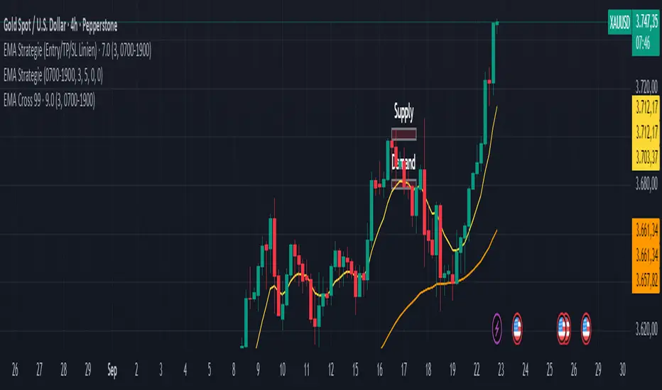
EMA Cross 99//@version=6
indicator("EMA Strategie (Indikator mit Entry/TP/SL)", overlay=true, max_lines_count=500, max_labels_count=500)
// === Inputs ===
rrRatio = input.float(3.0, "Risk:Reward (TP/SL)", minval=1.0, step=0.5)
sess = input.session("0700-1900", "Trading Session (lokal)")
// === EMAs ===
ema9 = ta.ema(close, 9)
ema50 = ta.ema(close, 50)
ema200 = ta.ema(close, 200)
// === Session ===
inSession = not na(time(timeframe.period, sess))
// === Trend + Cross ===
bullTrend = (ema9 > ema200) and (ema50 > ema200)
bearTrend = (ema9 < ema200) and (ema50 < ema200)
crossUp = ta.crossover(ema9, ema50)
crossDown = ta.crossunder(ema9, ema50)
// === Pullback Confirm ===
longTouch = bullTrend and crossUp and (low <= ema9)
longConfirm = longTouch and (close > open) and (close > ema9)
shortTouch = bearTrend and crossDown and (high >= ema9)
shortConfirm = shortTouch and (close < open) and (close < ema9)
// === Entry Signale ===
longEntry = longConfirm and inSession
shortEntry = shortConfirm and inSession
// === SL & TP Berechnung ===
longSL = ema50
longTP = close + (close - longSL) * rrRatio
shortSL = ema50
shortTP = close - (shortSL - close) * rrRatio
// === Long Markierungen ===
if (longEntry)
// Entry
line.new(bar_index, close, bar_index+20, close, color=color.green, style=line.style_dotted, width=2)
label.new(bar_index, close, "Entry", style=label.style_label_left, color=color.green, textcolor=color.white, size=size.tiny)
// TP
line.new(bar_index, longTP, bar_index+20, longTP, color=color.green, style=line.style_solid, width=2)
label.new(bar_index, longTP, "TP", style=label.style_label_left, color=color.green, textcolor=color.white, size=size.tiny)
// SL
line.new(bar_index, longSL, bar_index+20, longSL, color=color.red, style=line.style_solid, width=2)
label.new(bar_index, longSL, "SL", style=label.style_label_left, color=color.red, textcolor=color.white, size=size.tiny)
// === Short Markierungen ===
if (shortEntry)
// Entry
line.new(bar_index, close, bar_index+20, close, color=color.red, style=line.style_dotted, width=2)
label.new(bar_index, close, "Entry", style=label.style_label_left, color=color.red, textcolor=color.white, size=size.tiny)
// TP
line.new(bar_index, shortTP, bar_index+20, shortTP, color=color.red, style=line.style_solid, width=2)
label.new(bar_index, shortTP, "TP", style=label.style_label_left, color=color.red, textcolor=color.white, size=size.tiny)
// SL
line.new(bar_index, shortSL, bar_index+20, shortSL, color=color.green, style=line.style_solid, width=2)
label.new(bar_index, shortSL, "SL", style=label.style_label_left, color=color.green, textcolor=color.white, size=size.tiny)
// === EMAs anzeigen ===
plot(ema9, "EMA 9", color=color.yellow, linewidth=1)
plot(ema50, "EMA 50", color=color.orange, linewidth=1)
plot(ema200, "EMA 200", color=color.blue, linewidth=1)
// === Alerts ===
alertcondition(longEntry, title="Long Entry", message="EMA Strategie: LONG Einstiegssignal")
alertcondition(shortEntry, title="Short Entry", message="EMA Strategie: SHORT Einstiegssignal")
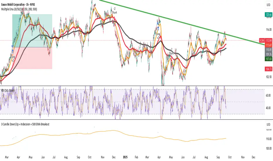
Parthiban Stock Market Buy V2 - Buy onlyFor BUY, condition
continuos 3 down candle
then forms Indecision candle
next candle close above Indecision candle
price above 500 EMA
For sell, condition
continuos 3 up candle
then forms Indecision candle
next candle close below Indecision candle
price below 500 EMA
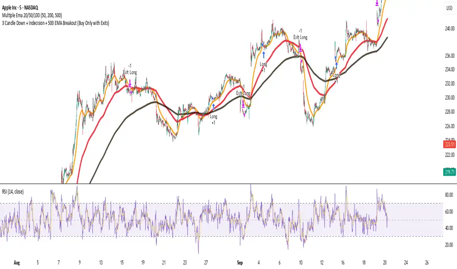
Parthiban - Stock Market BuyParthiban - Stock Market Buy
For BUY, condition
continuos 3 down candle
then forms Indecision candle
next candle close above Indecision candle
price above 500 EMA
For sell, condition
continuos 3 up candle
then forms Indecision candle
next candle close below Indecision candle
price below 500 EMA
Small Business Economic Conditions - Statistical Analysis ModelThe Small Business Economic Conditions Statistical Analysis Model (SBO-SAM) represents an econometric approach to measuring and analyzing the economic health of small business enterprises through multi-dimensional factor analysis and statistical methodologies. This indicator synthesizes eight fundamental economic components into a composite index that provides real-time assessment of small business operating conditions with statistical rigor. The model employs Z-score standardization, variance-weighted aggregation, higher-order moment analysis, and regime-switching detection to deliver comprehensive insights into small business economic conditions with statistical confidence intervals and multi-language accessibility.
1. Introduction and Theoretical Foundation
The development of quantitative models for assessing small business economic conditions has gained significant importance in contemporary financial analysis, particularly given the critical role small enterprises play in economic development and employment generation. Small businesses, typically defined as enterprises with fewer than 500 employees according to the U.S. Small Business Administration, constitute approximately 99.9% of all businesses in the United States and employ nearly half of the private workforce (U.S. Small Business Administration, 2024).
The theoretical framework underlying the SBO-SAM model draws extensively from established academic research in small business economics and quantitative finance. The foundational understanding of key drivers affecting small business performance builds upon the seminal work of Dunkelberg and Wade (2023) in their analysis of small business economic trends through the National Federation of Independent Business (NFIB) Small Business Economic Trends survey. Their research established the critical importance of optimism, hiring plans, capital expenditure intentions, and credit availability as primary determinants of small business performance.
The model incorporates insights from Federal Reserve Board research, particularly the Senior Loan Officer Opinion Survey (Federal Reserve Board, 2024), which demonstrates the critical importance of credit market conditions in small business operations. This research consistently shows that small businesses face disproportionate challenges during periods of credit tightening, as they typically lack access to capital markets and rely heavily on bank financing.
The statistical methodology employed in this model follows the econometric principles established by Hamilton (1989) in his work on regime-switching models and time series analysis. Hamilton's framework provides the theoretical foundation for identifying different economic regimes and understanding how economic relationships may vary across different market conditions. The variance-weighted aggregation technique draws from modern portfolio theory as developed by Markowitz (1952) and later refined by Sharpe (1964), applying these concepts to economic indicator construction rather than traditional asset allocation.
Additional theoretical support comes from the work of Engle and Granger (1987) on cointegration analysis, which provides the statistical framework for combining multiple time series while maintaining long-term equilibrium relationships. The model also incorporates insights from behavioral economics research by Kahneman and Tversky (1979) on prospect theory, recognizing that small business decision-making may exhibit systematic biases that affect economic outcomes.
2. Model Architecture and Component Structure
The SBO-SAM model employs eight orthogonalized economic factors that collectively capture the multifaceted nature of small business operating conditions. Each component is normalized using Z-score standardization with a rolling 252-day window, representing approximately one business year of trading data. This approach ensures statistical consistency across different market regimes and economic cycles, following the methodology established by Tsay (2010) in his treatment of financial time series analysis.
2.1 Small Cap Relative Performance Component
The first component measures the performance of the Russell 2000 index relative to the S&P 500, capturing the market-based assessment of small business equity valuations. This component reflects investor sentiment toward smaller enterprises and provides a forward-looking perspective on small business prospects. The theoretical justification for this component stems from the efficient market hypothesis as formulated by Fama (1970), which suggests that stock prices incorporate all available information about future prospects.
The calculation employs a 20-day rate of change with exponential smoothing to reduce noise while preserving signal integrity. The mathematical formulation is:
Small_Cap_Performance = (Russell_2000_t / S&P_500_t) / (Russell_2000_{t-20} / S&P_500_{t-20}) - 1
This relative performance measure eliminates market-wide effects and isolates the specific performance differential between small and large capitalization stocks, providing a pure measure of small business market sentiment.
2.2 Credit Market Conditions Component
Credit Market Conditions constitute the second component, incorporating commercial lending volumes and credit spread dynamics. This factor recognizes that small businesses are particularly sensitive to credit availability and borrowing costs, as established in numerous Federal Reserve studies (Bernanke and Gertler, 1995). Small businesses typically face higher borrowing costs and more stringent lending standards compared to larger enterprises, making credit conditions a critical determinant of their operating environment.
The model calculates credit spreads using high-yield bond ETFs relative to Treasury securities, providing a market-based measure of credit risk premiums that directly affect small business borrowing costs. The component also incorporates commercial and industrial loan growth data from the Federal Reserve's H.8 statistical release, which provides direct evidence of lending activity to businesses.
The mathematical specification combines these elements as:
Credit_Conditions = α₁ × (HYG_t / TLT_t) + α₂ × C&I_Loan_Growth_t
where HYG represents high-yield corporate bond ETF prices, TLT represents long-term Treasury ETF prices, and C&I_Loan_Growth represents the rate of change in commercial and industrial loans outstanding.
2.3 Labor Market Dynamics Component
The Labor Market Dynamics component captures employment cost pressures and labor availability metrics through the relationship between job openings and unemployment claims. This factor acknowledges that labor market tightness significantly impacts small business operations, as these enterprises typically have less flexibility in wage negotiations and face greater challenges in attracting and retaining talent during periods of low unemployment.
The theoretical foundation for this component draws from search and matching theory as developed by Mortensen and Pissarides (1994), which explains how labor market frictions affect employment dynamics. Small businesses often face higher search costs and longer hiring processes, making them particularly sensitive to labor market conditions.
The component is calculated as:
Labor_Tightness = Job_Openings_t / (Unemployment_Claims_t × 52)
This ratio provides a measure of labor market tightness, with higher values indicating greater difficulty in finding workers and potential wage pressures.
2.4 Consumer Demand Strength Component
Consumer Demand Strength represents the fourth component, combining consumer sentiment data with retail sales growth rates. Small businesses are disproportionately affected by consumer spending patterns, making this component crucial for assessing their operating environment. The theoretical justification comes from the permanent income hypothesis developed by Friedman (1957), which explains how consumer spending responds to both current conditions and future expectations.
The model weights consumer confidence and actual spending data to provide both forward-looking sentiment and contemporaneous demand indicators. The specification is:
Demand_Strength = β₁ × Consumer_Sentiment_t + β₂ × Retail_Sales_Growth_t
where β₁ and β₂ are determined through principal component analysis to maximize the explanatory power of the combined measure.
2.5 Input Cost Pressures Component
Input Cost Pressures form the fifth component, utilizing producer price index data to capture inflationary pressures on small business operations. This component is inversely weighted, recognizing that rising input costs negatively impact small business profitability and operating conditions. Small businesses typically have limited pricing power and face challenges in passing through cost increases to customers, making them particularly vulnerable to input cost inflation.
The theoretical foundation draws from cost-push inflation theory as described by Gordon (1988), which explains how supply-side price pressures affect business operations. The model employs a 90-day rate of change to capture medium-term cost trends while filtering out short-term volatility:
Cost_Pressure = -1 × (PPI_t / PPI_{t-90} - 1)
The negative weighting reflects the inverse relationship between input costs and business conditions.
2.6 Monetary Policy Impact Component
Monetary Policy Impact represents the sixth component, incorporating federal funds rates and yield curve dynamics. Small businesses are particularly sensitive to interest rate changes due to their higher reliance on variable-rate financing and limited access to capital markets. The theoretical foundation comes from monetary transmission mechanism theory as developed by Bernanke and Blinder (1992), which explains how monetary policy affects different segments of the economy.
The model calculates the absolute deviation of federal funds rates from a neutral 2% level, recognizing that both extremely low and high rates can create operational challenges for small enterprises. The yield curve component captures the shape of the term structure, which affects both borrowing costs and economic expectations:
Monetary_Impact = γ₁ × |Fed_Funds_Rate_t - 2.0| + γ₂ × (10Y_Yield_t - 2Y_Yield_t)
2.7 Currency Valuation Effects Component
Currency Valuation Effects constitute the seventh component, measuring the impact of US Dollar strength on small business competitiveness. A stronger dollar can benefit businesses with significant import components while disadvantaging exporters. The model employs Dollar Index volatility as a proxy for currency-related uncertainty that affects small business planning and operations.
The theoretical foundation draws from international trade theory and the work of Krugman (1987) on exchange rate effects on different business segments. Small businesses often lack hedging capabilities, making them more vulnerable to currency fluctuations:
Currency_Impact = -1 × DXY_Volatility_t
2.8 Regional Banking Health Component
The eighth and final component, Regional Banking Health, assesses the relative performance of regional banks compared to large financial institutions. Regional banks traditionally serve as primary lenders to small businesses, making their health a critical factor in small business credit availability and overall operating conditions.
This component draws from the literature on relationship banking as developed by Boot (2000), which demonstrates the importance of bank-borrower relationships, particularly for small enterprises. The calculation compares regional bank performance to large financial institutions:
Banking_Health = (Regional_Banks_Index_t / Large_Banks_Index_t) - 1
3. Statistical Methodology and Advanced Analytics
The model employs statistical techniques to ensure robustness and reliability. Z-score normalization is applied to each component using rolling 252-day windows, providing standardized measures that remain consistent across different time periods and market conditions. This approach follows the methodology established by Engle and Granger (1987) in their cointegration analysis framework.
3.1 Variance-Weighted Aggregation
The composite index calculation utilizes variance-weighted aggregation, where component weights are determined by the inverse of their historical variance. This approach, derived from modern portfolio theory, ensures that more stable components receive higher weights while reducing the impact of highly volatile factors. The mathematical formulation follows the principle that optimal weights are inversely proportional to variance, maximizing the signal-to-noise ratio of the composite indicator.
The weight for component i is calculated as:
w_i = (1/σᵢ²) / Σⱼ(1/σⱼ²)
where σᵢ² represents the variance of component i over the lookback period.
3.2 Higher-Order Moment Analysis
Higher-order moment analysis extends beyond traditional mean and variance calculations to include skewness and kurtosis measurements. Skewness provides insight into the asymmetry of the sentiment distribution, while kurtosis measures the tail behavior and potential for extreme events. These metrics offer valuable information about the underlying distribution characteristics and potential regime changes.
Skewness is calculated as:
Skewness = E / σ³
Kurtosis is calculated as:
Kurtosis = E / σ⁴ - 3
where μ represents the mean and σ represents the standard deviation of the distribution.
3.3 Regime-Switching Detection
The model incorporates regime-switching detection capabilities based on the Hamilton (1989) framework. This allows for identification of different economic regimes characterized by distinct statistical properties. The regime classification employs percentile-based thresholds:
- Regime 3 (Very High): Percentile rank > 80
- Regime 2 (High): Percentile rank 60-80
- Regime 1 (Moderate High): Percentile rank 50-60
- Regime 0 (Neutral): Percentile rank 40-50
- Regime -1 (Moderate Low): Percentile rank 30-40
- Regime -2 (Low): Percentile rank 20-30
- Regime -3 (Very Low): Percentile rank < 20
3.4 Information Theory Applications
The model incorporates information theory concepts, specifically Shannon entropy measurement, to assess the information content of the sentiment distribution. Shannon entropy, as developed by Shannon (1948), provides a measure of the uncertainty or information content in a probability distribution:
H(X) = -Σᵢ p(xᵢ) log₂ p(xᵢ)
Higher entropy values indicate greater unpredictability and information content in the sentiment series.
3.5 Long-Term Memory Analysis
The Hurst exponent calculation provides insight into the long-term memory characteristics of the sentiment series. Originally developed by Hurst (1951) for analyzing Nile River flow patterns, this measure has found extensive application in financial time series analysis. The Hurst exponent H is calculated using the rescaled range statistic:
H = log(R/S) / log(T)
where R/S represents the rescaled range and T represents the time period. Values of H > 0.5 indicate long-term positive autocorrelation (persistence), while H < 0.5 indicates mean-reverting behavior.
3.6 Structural Break Detection
The model employs Chow test approximation for structural break detection, based on the methodology developed by Chow (1960). This technique identifies potential structural changes in the underlying relationships by comparing the stability of regression parameters across different time periods:
Chow_Statistic = (RSS_restricted - RSS_unrestricted) / RSS_unrestricted × (n-2k)/k
where RSS represents residual sum of squares, n represents sample size, and k represents the number of parameters.
4. Implementation Parameters and Configuration
4.1 Language Selection Parameters
The model provides comprehensive multi-language support across five languages: English, German (Deutsch), Spanish (Español), French (Français), and Japanese (日本語). This feature enhances accessibility for international users and ensures cultural appropriateness in terminology usage. The language selection affects all internal displays, statistical classifications, and alert messages while maintaining consistency in underlying calculations.
4.2 Model Configuration Parameters
Calculation Method: Users can select from four aggregation methodologies:
- Equal-Weighted: All components receive identical weights
- Variance-Weighted: Components weighted inversely to their historical variance
- Principal Component: Weights determined through principal component analysis
- Dynamic: Adaptive weighting based on recent performance
Sector Specification: The model allows for sector-specific calibration:
- General: Broad-based small business assessment
- Retail: Emphasis on consumer demand and seasonal factors
- Manufacturing: Enhanced weighting of input costs and currency effects
- Services: Focus on labor market dynamics and consumer demand
- Construction: Emphasis on credit conditions and monetary policy
Lookback Period: Statistical analysis window ranging from 126 to 504 trading days, with 252 days (one business year) as the optimal default based on academic research.
Smoothing Period: Exponential moving average period from 1 to 21 days, with 5 days providing optimal noise reduction while preserving signal integrity.
4.3 Statistical Threshold Parameters
Upper Statistical Boundary: Configurable threshold between 60-80 (default 70) representing the upper significance level for regime classification.
Lower Statistical Boundary: Configurable threshold between 20-40 (default 30) representing the lower significance level for regime classification.
Statistical Significance Level (α): Alpha level for statistical tests, configurable between 0.01-0.10 with 0.05 as the standard academic default.
4.4 Display and Visualization Parameters
Color Theme Selection: Eight professional color schemes optimized for different user preferences and accessibility requirements:
- Gold: Traditional financial industry colors
- EdgeTools: Professional blue-gray scheme
- Behavioral: Psychology-based color mapping
- Quant: Value-based quantitative color scheme
- Ocean: Blue-green maritime theme
- Fire: Warm red-orange theme
- Matrix: Green-black technology theme
- Arctic: Cool blue-white theme
Dark Mode Optimization: Automatic color adjustment for dark chart backgrounds, ensuring optimal readability across different viewing conditions.
Line Width Configuration: Main index line thickness adjustable from 1-5 pixels for optimal visibility.
Background Intensity: Transparency control for statistical regime backgrounds, adjustable from 90-99% for subtle visual enhancement without distraction.
4.5 Alert System Configuration
Alert Frequency Options: Three frequency settings to match different trading styles:
- Once Per Bar: Single alert per bar formation
- Once Per Bar Close: Alert only on confirmed bar close
- All: Continuous alerts for real-time monitoring
Statistical Extreme Alerts: Notifications when the index reaches 99% confidence levels (Z-score > 2.576 or < -2.576).
Regime Transition Alerts: Notifications when statistical boundaries are crossed, indicating potential regime changes.
5. Practical Application and Interpretation Guidelines
5.1 Index Interpretation Framework
The SBO-SAM index operates on a 0-100 scale with statistical normalization ensuring consistent interpretation across different time periods and market conditions. Values above 70 indicate statistically elevated small business conditions, suggesting favorable operating environment with potential for expansion and growth. Values below 30 indicate statistically reduced conditions, suggesting challenging operating environment with potential constraints on business activity.
The median reference line at 50 represents the long-term equilibrium level, with deviations providing insight into cyclical conditions relative to historical norms. The statistical confidence bands at 95% levels (approximately ±2 standard deviations) help identify when conditions reach statistically significant extremes.
5.2 Regime Classification System
The model employs a seven-level regime classification system based on percentile rankings:
Very High Regime (P80+): Exceptional small business conditions, typically associated with strong economic growth, easy credit availability, and favorable regulatory environment. Historical analysis suggests these periods often precede economic peaks and may warrant caution regarding sustainability.
High Regime (P60-80): Above-average conditions supporting business expansion and investment. These periods typically feature moderate growth, stable credit conditions, and positive consumer sentiment.
Moderate High Regime (P50-60): Slightly above-normal conditions with mixed signals. Careful monitoring of individual components helps identify emerging trends.
Neutral Regime (P40-50): Balanced conditions near long-term equilibrium. These periods often represent transition phases between different economic cycles.
Moderate Low Regime (P30-40): Slightly below-normal conditions with emerging headwinds. Early warning signals may appear in credit conditions or consumer demand.
Low Regime (P20-30): Below-average conditions suggesting challenging operating environment. Businesses may face constraints on growth and expansion.
Very Low Regime (P0-20): Severely constrained conditions, typically associated with economic recessions or financial crises. These periods often present opportunities for contrarian positioning.
5.3 Component Analysis and Diagnostics
Individual component analysis provides valuable diagnostic information about the underlying drivers of overall conditions. Divergences between components can signal emerging trends or structural changes in the economy.
Credit-Labor Divergence: When credit conditions improve while labor markets tighten, this may indicate early-stage economic acceleration with potential wage pressures.
Demand-Cost Divergence: Strong consumer demand coupled with rising input costs suggests inflationary pressures that may constrain small business margins.
Market-Fundamental Divergence: Disconnection between small-cap equity performance and fundamental conditions may indicate market inefficiencies or changing investor sentiment.
5.4 Temporal Analysis and Trend Identification
The model provides multiple temporal perspectives through momentum analysis, rate of change calculations, and trend decomposition. The 20-day momentum indicator helps identify short-term directional changes, while the Hodrick-Prescott filter approximation separates cyclical components from long-term trends.
Acceleration analysis through second-order momentum calculations provides early warning signals for potential trend reversals. Positive acceleration during declining conditions may indicate approaching inflection points, while negative acceleration during improving conditions may suggest momentum loss.
5.5 Statistical Confidence and Uncertainty Quantification
The model provides comprehensive uncertainty quantification through confidence intervals, volatility measures, and regime stability analysis. The 95% confidence bands help users understand the statistical significance of current readings and identify when conditions reach historically extreme levels.
Volatility analysis provides insight into the stability of current conditions, with higher volatility indicating greater uncertainty and potential for rapid changes. The regime stability measure, calculated as the inverse of volatility, helps assess the sustainability of current conditions.
6. Risk Management and Limitations
6.1 Model Limitations and Assumptions
The SBO-SAM model operates under several important assumptions that users must understand for proper interpretation. The model assumes that historical relationships between economic variables remain stable over time, though the regime-switching framework helps accommodate some structural changes. The 252-day lookback period provides reasonable statistical power while maintaining sensitivity to changing conditions, but may not capture longer-term structural shifts.
The model's reliance on publicly available economic data introduces inherent lags in some components, particularly those based on government statistics. Users should consider these timing differences when interpreting real-time conditions. Additionally, the model's focus on quantitative factors may not fully capture qualitative factors such as regulatory changes, geopolitical events, or technological disruptions that could significantly impact small business conditions.
The model's timeframe restrictions ensure statistical validity by preventing application to intraday periods where the underlying economic relationships may be distorted by market microstructure effects, trading noise, and temporal misalignment with the fundamental data sources. Users must utilize daily or longer timeframes to ensure the model's statistical foundations remain valid and interpretable.
6.2 Data Quality and Reliability Considerations
The model's accuracy depends heavily on the quality and availability of underlying economic data. Market-based components such as equity indices and bond prices provide real-time information but may be subject to short-term volatility unrelated to fundamental conditions. Economic statistics provide more stable fundamental information but may be subject to revisions and reporting delays.
Users should be aware that extreme market conditions may temporarily distort some components, particularly those based on financial market data. The model's statistical normalization helps mitigate these effects, but users should exercise additional caution during periods of market stress or unusual volatility.
6.3 Interpretation Caveats and Best Practices
The SBO-SAM model provides statistical analysis and should not be interpreted as investment advice or predictive forecasting. The model's output represents an assessment of current conditions based on historical relationships and may not accurately predict future outcomes. Users should combine the model's insights with other analytical tools and fundamental analysis for comprehensive decision-making.
The model's regime classifications are based on historical percentile rankings and may not fully capture the unique characteristics of current economic conditions. Users should consider the broader economic context and potential structural changes when interpreting regime classifications.
7. Academic References and Bibliography
Bernanke, B. S., & Blinder, A. S. (1992). The Federal Funds Rate and the Channels of Monetary Transmission. American Economic Review, 82(4), 901-921.
Bernanke, B. S., & Gertler, M. (1995). Inside the Black Box: The Credit Channel of Monetary Policy Transmission. Journal of Economic Perspectives, 9(4), 27-48.
Boot, A. W. A. (2000). Relationship Banking: What Do We Know? Journal of Financial Intermediation, 9(1), 7-25.
Chow, G. C. (1960). Tests of Equality Between Sets of Coefficients in Two Linear Regressions. Econometrica, 28(3), 591-605.
Dunkelberg, W. C., & Wade, H. (2023). NFIB Small Business Economic Trends. National Federation of Independent Business Research Foundation, Washington, D.C.
Engle, R. F., & Granger, C. W. J. (1987). Co-integration and Error Correction: Representation, Estimation, and Testing. Econometrica, 55(2), 251-276.
Fama, E. F. (1970). Efficient Capital Markets: A Review of Theory and Empirical Work. Journal of Finance, 25(2), 383-417.
Federal Reserve Board. (2024). Senior Loan Officer Opinion Survey on Bank Lending Practices. Board of Governors of the Federal Reserve System, Washington, D.C.
Friedman, M. (1957). A Theory of the Consumption Function. Princeton University Press, Princeton, NJ.
Gordon, R. J. (1988). The Role of Wages in the Inflation Process. American Economic Review, 78(2), 276-283.
Hamilton, J. D. (1989). A New Approach to the Economic Analysis of Nonstationary Time Series and the Business Cycle. Econometrica, 57(2), 357-384.
Hurst, H. E. (1951). Long-term Storage Capacity of Reservoirs. Transactions of the American Society of Civil Engineers, 116(1), 770-799.
Kahneman, D., & Tversky, A. (1979). Prospect Theory: An Analysis of Decision under Risk. Econometrica, 47(2), 263-291.
Krugman, P. (1987). Pricing to Market When the Exchange Rate Changes. In S. W. Arndt & J. D. Richardson (Eds.), Real-Financial Linkages among Open Economies (pp. 49-70). MIT Press, Cambridge, MA.
Markowitz, H. (1952). Portfolio Selection. Journal of Finance, 7(1), 77-91.
Mortensen, D. T., & Pissarides, C. A. (1994). Job Creation and Job Destruction in the Theory of Unemployment. Review of Economic Studies, 61(3), 397-415.
Shannon, C. E. (1948). A Mathematical Theory of Communication. Bell System Technical Journal, 27(3), 379-423.
Sharpe, W. F. (1964). Capital Asset Prices: A Theory of Market Equilibrium under Conditions of Risk. Journal of Finance, 19(3), 425-442.
Tsay, R. S. (2010). Analysis of Financial Time Series (3rd ed.). John Wiley & Sons, Hoboken, NJ.
U.S. Small Business Administration. (2024). Small Business Profile. Office of Advocacy, Washington, D.C.
8. Technical Implementation Notes
The SBO-SAM model is implemented in Pine Script version 6 for the TradingView platform, ensuring compatibility with modern charting and analysis tools. The implementation follows best practices for financial indicator development, including proper error handling, data validation, and performance optimization.
The model includes comprehensive timeframe validation to ensure statistical accuracy and reliability. The indicator operates exclusively on daily (1D) timeframes or higher, including weekly (1W), monthly (1M), and longer periods. This restriction ensures that the statistical analysis maintains appropriate temporal resolution for the underlying economic data sources, which are primarily reported on daily or longer intervals.
When users attempt to apply the model to intraday timeframes (such as 1-minute, 5-minute, 15-minute, 30-minute, 1-hour, 2-hour, 4-hour, 6-hour, 8-hour, or 12-hour charts), the system displays a comprehensive error message in the user's selected language and prevents execution. This safeguard protects users from potentially misleading results that could occur when applying daily-based economic analysis to shorter timeframes where the underlying data relationships may not hold.
The model's statistical calculations are performed using vectorized operations where possible to ensure computational efficiency. The multi-language support system employs Unicode character encoding to ensure proper display of international characters across different platforms and devices.
The alert system utilizes TradingView's native alert functionality, providing users with flexible notification options including email, SMS, and webhook integrations. The alert messages include comprehensive statistical information to support informed decision-making.
The model's visualization system employs professional color schemes designed for optimal readability across different chart backgrounds and display devices. The system includes dynamic color transitions based on momentum and volatility, professional glow effects for enhanced line visibility, and transparency controls that allow users to customize the visual intensity to match their preferences and analytical requirements. The clean confidence band implementation provides clear statistical boundaries without visual distractions, maintaining focus on the analytical content.

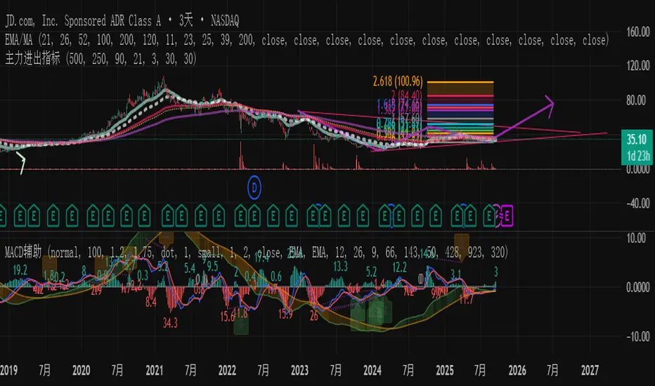
主力资金进出监控器Main Capital Flow Monitor-MEWINSIGHTMain Capital Flow Monitor Indicator
Indicator Description
This indicator utilizes a multi-cycle composite weighting algorithm to accurately capture the movement of main capital in and out of key price zones. The core logic is built upon three dimensions:
Multi-Cycle Pressure/Support System
Using triple timeframes (500-day/250-day/90-day) to calculate:
Long-term resistance lines (VAR1-3): Monitoring historical high resistance zones
Long-term support lines (VAR4-6): Identifying historical low support zones
EMA21 smoothing is applied to eliminate short-term fluctuations
Dynamic Capital Activity Engine
Proprietary VARD volatility algorithm:
VARD = EMA
Automatically amplifies volatility sensitivity by 10x when price approaches the safety margin (VARA×1.35), precisely capturing abnormal main capital movements
Capital Inflow Trigger Mechanism
Capital entry signals require simultaneous fulfillment of:
Price touching 30-day low zone (VARE)
Capital activity breaking recent peaks (VARF)
Weighted capital flow verified through triple EMA:
Capital Entry = EMA / 618
Visualization:
Green histogram: Continuous main capital inflow
Red histogram: Abnormal daily capital movement intensity
Column height intuitively displays capital strength
Application Scenarios:
Consecutive green columns → Main capital accumulation at bottom
Sudden expansion of red columns → Abnormal main capital rush
Continuous fluctuations near zero axis → Main capital washing phase
Core Value:
Provides 1-3 trading days early warning of main capital movements, suitable for:
Medium/long-term investors identifying main capital accumulation zones
Short-term traders capturing abnormal main capital breakouts
Risk control avoiding main capital distribution phases
Parameter Notes: Default parameters are optimized through historical A-share market backtesting. Users can adjust cycle parameters according to different market characteristics (suggest extending cycles by 20% for European/American markets).
Formula Features:
Multi-timeframe weighted synthesis technology
Dynamic sensitivity adjustment mechanism
Main capital activity intensity quantification
Early warning function for capital movements
Suitable Markets:
Stocks, futures, cryptocurrencies and other financial markets with obvious main capital characteristics.
指标名称:主力资金进出监控器
指标描述:
本指标通过多周期复合加权算法,精准捕捉主力资金在关键价格区域的进出动向。核心逻辑基于三大维度构建:
多周期压力/支撑体系
通过500日/250日/90日三重时间框架,分别计算:
长期压力线(VAR1-3):监控历史高位阻力区
长期支撑线(VAR4-6):识别历史低位承接区
采用EMA21平滑处理,消除短期波动干扰
动态资金活跃度引擎
独创VARD波动率算法:
当价格接近安全边际(VARA×1.35)时自动放大波动敏感度10倍,精准捕捉主力异动
资金进场触发机制
资金入场信号需同时满足:
价格触及30日最低区域(VARE)
资金活跃度突破近期峰值(VARF)
通过三重EMA验证的加权资金流:
资金入场 = EMA / 618
可视化呈现:
绿色柱状图:主力资金持续流入
红色柱状图:当日资金异动量级
柱体高度直观显示资金强度
使用场景:
绿色柱体连续出现 → 主力底部吸筹
红色柱体突然放大 → 主力异动抢筹
零轴附近持续波动 → 主力洗盘阶段
核心价值:
提前1-3个交易日预警主力资金动向,适用于:
中长线投资者识别主力建仓区间
短线交易者捕捉主力异动突破
风险控制规避主力出货阶段
参数说明:默认参数经A股历史数据回测优化,用户可根据不同市场特性调整周期参数(建议欧美市场延长周期20%)
Relative Strength vs. Benchmark (相對強度)This "Relative Strength vs. Benchmark" indicator helps you see a stock's true performance against a benchmark (like the S&P 500) at a glance. By calculating the price ratio between the two, it strips away the overall market noise, allowing you to focus on identifying true market leaders and underperforming laggards.
How It Works
Core Formula: Relative Strength = Stock Price / Benchmark Index Price
A Rising Line: Means the stock is outperforming the benchmark.
A Falling Line: Means the stock is underperforming the benchmark.
The indicator also includes a Moving Average (MA) of the Relative Strength line itself. This MA helps to confirm the trend of relative strength and filter out short-term noise.
How to Use
Find Market Leaders: When the market is in an uptrend or consolidating, look for stocks whose RS line is breaking out to new highs.
Avoid Laggards: If the RS line is consistently below its moving average or making new lows, the stock is significantly underperforming the market and should be treated with caution.
Trend Change Signals: A cross of the RS line above its MA can be seen as a signal that a new trend of relative outperformance is beginning. A cross below suggests the trend is weakening.
Features & Settings
Customizable Benchmark: You can change the default benchmark from TWSE:TSE to any symbol you need, such as SP:SPX for the S&P 500 or NASDAQ:NDX for the Nasdaq 100.
Adjustable MA Length: Customize the period for the RS Moving Average to fit your trading style (short-term or long-term).
Visual Toggle: Easily turn the colored background fill on or off according to your preference.
Hope you find this tool helpful in your analysis!
Bar Index & TimeLibrary to convert a bar index to a timestamp and vice versa.
Utilizes runtime memory to store the 𝚝𝚒𝚖𝚎 and 𝚝𝚒𝚖𝚎_𝚌𝚕𝚘𝚜𝚎 values of every bar on the chart (and optional future bars), with the ability of storing additional custom values for every chart bar.
█ PREFACE
This library aims to tackle some problems that pine coders (from beginners to advanced) often come across, such as:
I'm trying to draw an object with a 𝚋𝚊𝚛_𝚒𝚗𝚍𝚎𝚡 that is more than 10,000 bars into the past, but this causes my script to fail. How can I convert the 𝚋𝚊𝚛_𝚒𝚗𝚍𝚎𝚡 to a UNIX time so that I can draw visuals using xloc.bar_time ?
I have a diagonal line drawing and I want to get the "y" value at a specific time, but line.get_price() only accepts a bar index value. How can I convert the timestamp into a bar index value so that I can still use this function?
I want to get a previous 𝚘𝚙𝚎𝚗 value that occurred at a specific timestamp. How can I convert the timestamp into a historical offset so that I can use 𝚘𝚙𝚎𝚗 ?
I want to reference a very old value for a variable. How can I access a previous value that is older than the maximum historical buffer size of 𝚟𝚊𝚛𝚒𝚊𝚋𝚕𝚎 ?
This library can solve the above problems (and many more) with the addition of a few lines of code, rather than requiring the coder to refactor their script to accommodate the limitations.
█ OVERVIEW
The core functionality provided is conversion between xloc.bar_index and xloc.bar_time values.
The main component of the library is the 𝙲𝚑𝚊𝚛𝚝𝙳𝚊𝚝𝚊 object, created via the 𝚌𝚘𝚕𝚕𝚎𝚌𝚝𝙲𝚑𝚊𝚛𝚝𝙳𝚊𝚝𝚊() function which basically stores the 𝚝𝚒𝚖𝚎 and 𝚝𝚒𝚖𝚎_𝚌𝚕𝚘𝚜𝚎 of every bar on the chart, and there are 3 more overloads to this function that allow collecting and storing additional data. Once a 𝙲𝚑𝚊𝚛𝚝𝙳𝚊𝚝𝚊 object is created, use any of the exported methods:
Methods to convert a UNIX timestamp into a bar index or bar offset:
𝚝𝚒𝚖𝚎𝚜𝚝𝚊𝚖𝚙𝚃𝚘𝙱𝚊𝚛𝙸𝚗𝚍𝚎𝚡(), 𝚐𝚎𝚝𝙽𝚞𝚖𝚋𝚎𝚛𝙾𝚏𝙱𝚊𝚛𝚜𝙱𝚊𝚌𝚔()
Methods to retrieve the stored data for a bar index:
𝚝𝚒𝚖𝚎𝙰𝚝𝙱𝚊𝚛𝙸𝚗𝚍𝚎𝚡(), 𝚝𝚒𝚖𝚎𝙲𝚕𝚘𝚜𝚎𝙰𝚝𝙱𝚊𝚛𝙸𝚗𝚍𝚎𝚡(), 𝚟𝚊𝚕𝚞𝚎𝙰𝚝𝙱𝚊𝚛𝙸𝚗𝚍𝚎𝚡(), 𝚐𝚎𝚝𝙰𝚕𝚕𝚅𝚊𝚛𝚒𝚊𝚋𝚕𝚎𝚜𝙰𝚝𝙱𝚊𝚛𝙸𝚗𝚍𝚎𝚡()
Methods to retrieve the stored data at a number of bars back (i.e., historical offset):
𝚝𝚒𝚖𝚎(), 𝚝𝚒𝚖𝚎𝙲𝚕𝚘𝚜𝚎(), 𝚟𝚊𝚕𝚞𝚎()
Methods to retrieve all the data points from the earliest bar (or latest bar) stored in memory, which can be useful for debugging purposes:
𝚐𝚎𝚝𝙴𝚊𝚛𝚕𝚒𝚎𝚜𝚝𝚂𝚝𝚘𝚛𝚎𝚍𝙳𝚊𝚝𝚊(), 𝚐𝚎𝚝𝙻𝚊𝚝𝚎𝚜𝚝𝚂𝚝𝚘𝚛𝚎𝚍𝙳𝚊𝚝𝚊()
Note: the library's strong suit is referencing data from very old bars in the past, which is especially useful for scripts that perform its necessary calculations only on the last bar.
█ USAGE
Step 1
Import the library. Replace with the latest available version number for this library.
//@version=6
indicator("Usage")
import n00btraders/ChartData/
Step 2
Create a 𝙲𝚑𝚊𝚛𝚝𝙳𝚊𝚝𝚊 object to collect data on every bar. Do not declare as `var` or `varip`.
chartData = ChartData.collectChartData() // call on every bar to accumulate the necessary data
Step 3
Call any method(s) on the 𝙲𝚑𝚊𝚛𝚝𝙳𝚊𝚝𝚊 object. Do not modify its fields directly.
if barstate.islast
int firstBarTime = chartData.timeAtBarIndex(0)
int lastBarTime = chartData.time(0)
log.info("First `time`: " + str.format_time(firstBarTime) + ", Last `time`: " + str.format_time(lastBarTime))
█ EXAMPLES
• Collect Future Times
The overloaded 𝚌𝚘𝚕𝚕𝚎𝚌𝚝𝙲𝚑𝚊𝚛𝚝𝙳𝚊𝚝𝚊() functions that accept a 𝚋𝚊𝚛𝚜𝙵𝚘𝚛𝚠𝚊𝚛𝚍 argument can additionally store time values for up to 500 bars into the future.
//@version=6
indicator("Example `collectChartData(barsForward)`")
import n00btraders/ChartData/1
chartData = ChartData.collectChartData(barsForward = 500)
var rectangle = box.new(na, na, na, na, xloc = xloc.bar_time, force_overlay = true)
if barstate.islast
int futureTime = chartData.timeAtBarIndex(bar_index + 100)
int lastBarTime = time
box.set_lefttop(rectangle, lastBarTime, open)
box.set_rightbottom(rectangle, futureTime, close)
box.set_text(rectangle, "Extending box 100 bars to the right. Time: " + str.format_time(futureTime))
• Collect Custom Data
The overloaded 𝚌𝚘𝚕𝚕𝚎𝚌𝚝𝙲𝚑𝚊𝚛𝚝𝙳𝚊𝚝𝚊() functions that accept a 𝚟𝚊𝚛𝚒𝚊𝚋𝚕𝚎𝚜 argument can additionally store custom user-specified values for every bar on the chart.
//@version=6
indicator("Example `collectChartData(variables)`")
import n00btraders/ChartData/1
var map variables = map.new()
variables.put("open", open)
variables.put("close", close)
variables.put("open-close midpoint", (open + close) / 2)
variables.put("boolean", open > close ? 1 : 0)
chartData = ChartData.collectChartData(variables = variables)
var fgColor = chart.fg_color
var table1 = table.new(position.top_right, 2, 9, color(na), fgColor, 1, fgColor, 1, true)
var table2 = table.new(position.bottom_right, 2, 9, color(na), fgColor, 1, fgColor, 1, true)
if barstate.isfirst
table.cell(table1, 0, 0, "ChartData.value()", text_color = fgColor)
table.cell(table2, 0, 0, "open ", text_color = fgColor)
table.merge_cells(table1, 0, 0, 1, 0)
table.merge_cells(table2, 0, 0, 1, 0)
for i = 1 to 8
table.cell(table1, 0, i, text_color = fgColor, text_halign = text.align_left, text_font_family = font.family_monospace)
table.cell(table2, 0, i, text_color = fgColor, text_halign = text.align_left, text_font_family = font.family_monospace)
table.cell(table1, 1, i, text_color = fgColor)
table.cell(table2, 1, i, text_color = fgColor)
if barstate.islast
for i = 1 to 8
float open1 = chartData.value("open", 5000 * i)
float open2 = i < 3 ? open : -1
table.cell_set_text(table1, 0, i, "chartData.value(\"open\", " + str.tostring(5000 * i) + "): ")
table.cell_set_text(table2, 0, i, "open : ")
table.cell_set_text(table1, 1, i, str.tostring(open1))
table.cell_set_text(table2, 1, i, open2 >= 0 ? str.tostring(open2) : "Error")
• xloc.bar_index → xloc.bar_time
The 𝚝𝚒𝚖𝚎 value (or 𝚝𝚒𝚖𝚎_𝚌𝚕𝚘𝚜𝚎 value) can be retrieved for any bar index that is stored in memory by the 𝙲𝚑𝚊𝚛𝚝𝙳𝚊𝚝𝚊 object.
//@version=6
indicator("Example `timeAtBarIndex()`")
import n00btraders/ChartData/1
chartData = ChartData.collectChartData()
if barstate.islast
int start = bar_index - 15000
int end = bar_index - 100
// line.new(start, close, end, close) // !ERROR - `start` value is too far from current bar index
start := chartData.timeAtBarIndex(start)
end := chartData.timeAtBarIndex(end)
line.new(start, close, end, close, xloc.bar_time, width = 10)
• xloc.bar_time → xloc.bar_index
Use 𝚝𝚒𝚖𝚎𝚜𝚝𝚊𝚖𝚙𝚃𝚘𝙱𝚊𝚛𝙸𝚗𝚍𝚎𝚡() to find the bar that a timestamp belongs to.
If the timestamp falls in between the close of one bar and the open of the next bar,
the 𝚜𝚗𝚊𝚙 parameter can be used to determine which bar to choose:
𝚂𝚗𝚊𝚙.𝙻𝙴𝙵𝚃 - prefer to choose the leftmost bar (typically used for closing times)
𝚂𝚗𝚊𝚙.𝚁𝙸𝙶𝙷𝚃 - prefer to choose the rightmost bar (typically used for opening times)
𝚂𝚗𝚊𝚙.𝙳𝙴𝙵𝙰𝚄𝙻𝚃 (or 𝚗𝚊) - copies the same behavior as xloc.bar_time uses for drawing objects
//@version=6
indicator("Example `timestampToBarIndex()`")
import n00btraders/ChartData/1
startTimeInput = input.time(timestamp("01 Aug 2025 08:30 -0500"), "Session Start Time")
endTimeInput = input.time(timestamp("01 Aug 2025 15:15 -0500"), "Session End Time")
chartData = ChartData.collectChartData()
if barstate.islastconfirmedhistory
int startBarIndex = chartData.timestampToBarIndex(startTimeInput, ChartData.Snap.RIGHT)
int endBarIndex = chartData.timestampToBarIndex(endTimeInput, ChartData.Snap.LEFT)
line1 = line.new(startBarIndex, 0, startBarIndex, 1, extend = extend.both, color = color.new(color.green, 60), force_overlay = true)
line2 = line.new(endBarIndex, 0, endBarIndex, 1, extend = extend.both, color = color.new(color.green, 60), force_overlay = true)
linefill.new(line1, line2, color.new(color.green, 90))
// using Snap.DEFAULT to show that it is equivalent to drawing lines using `xloc.bar_time` (i.e., it aligns to the same bars)
startBarIndex := chartData.timestampToBarIndex(startTimeInput)
endBarIndex := chartData.timestampToBarIndex(endTimeInput)
line.new(startBarIndex, 0, startBarIndex, 1, extend = extend.both, color = color.yellow, width = 3)
line.new(endBarIndex, 0, endBarIndex, 1, extend = extend.both, color = color.yellow, width = 3)
line.new(startTimeInput, 0, startTimeInput, 1, xloc.bar_time, extend.both, color.new(color.blue, 85), width = 11)
line.new(endTimeInput, 0, endTimeInput, 1, xloc.bar_time, extend.both, color.new(color.blue, 85), width = 11)
• Get Price of Line at Timestamp
The pine script built-in function line.get_price() requires working with bar index values. To get the price of a line in terms of a timestamp, convert the timestamp into a bar index or offset.
//@version=6
indicator("Example `line.get_price()` at timestamp")
import n00btraders/ChartData/1
lineStartInput = input.time(timestamp("01 Aug 2025 08:30 -0500"), "Line Start")
chartData = ChartData.collectChartData()
var diagonal = line.new(na, na, na, na, force_overlay = true)
if time <= lineStartInput
line.set_xy1(diagonal, bar_index, open)
if barstate.islastconfirmedhistory
line.set_xy2(diagonal, bar_index, close)
if barstate.islast
int timeOneWeekAgo = timenow - (7 * timeframe.in_seconds("1D") * 1000)
// Note: could also use `timetampToBarIndex(timeOneWeekAgo, Snap.DEFAULT)` and pass the value directly to `line.get_price()`
int barsOneWeekAgo = chartData.getNumberOfBarsBack(timeOneWeekAgo)
float price = line.get_price(diagonal, bar_index - barsOneWeekAgo)
string formatString = "Time 1 week ago: {0,number,#}\n - Equivalent to {1} bars ago\n\n𝚕𝚒𝚗𝚎.𝚐𝚎𝚝_𝚙𝚛𝚒𝚌𝚎(): {2,number,#.##}"
string labelText = str.format(formatString, timeOneWeekAgo, barsOneWeekAgo, price)
label.new(timeOneWeekAgo, price, labelText, xloc.bar_time, style = label.style_label_lower_right, size = 16, textalign = text.align_left, force_overlay = true)
█ RUNTIME ERROR MESSAGES
This library's functions will generate a custom runtime error message in the following cases:
𝚌𝚘𝚕𝚕𝚎𝚌𝚝𝙲𝚑𝚊𝚛𝚝𝙳𝚊𝚝𝚊() is not called consecutively, or is called more than once on a single bar
Invalid 𝚋𝚊𝚛𝚜𝙵𝚘𝚛𝚠𝚊𝚛𝚍 argument in the 𝚌𝚘𝚕𝚕𝚎𝚌𝚝𝙲𝚑𝚊𝚛𝚝𝙳𝚊𝚝𝚊() function
Invalid 𝚟𝚊𝚛𝚒𝚊𝚋𝚕𝚎𝚜 argument in the 𝚌𝚘𝚕𝚕𝚎𝚌𝚝𝙲𝚑𝚊𝚛𝚝𝙳𝚊𝚝𝚊() function
Invalid 𝚕𝚎𝚗𝚐𝚝𝚑 argument in any of the functions that accept a number of bars back
Note: there is no runtime error generated for an invalid 𝚝𝚒𝚖𝚎𝚜𝚝𝚊𝚖𝚙 or 𝚋𝚊𝚛𝙸𝚗𝚍𝚎𝚡 argument in any of the functions. Instead, the functions will assign 𝚗𝚊 to the returned values.
Any other runtime errors are due to incorrect usage of the library.
█ NOTES
• Function Descriptions
The library source code uses Markdown for the exported functions. Hover over a function/method call in the Pine Editor to display formatted, detailed information about the function/method.
//@version=6
indicator("Demo Function Tooltip")
import n00btraders/ChartData/1
chartData = ChartData.collectChartData()
int barIndex = chartData.timestampToBarIndex(timenow)
log.info(str.tostring(barIndex))
• Historical vs. Realtime Behavior
Under the hood, the data collector for this library is declared as `var`. Because of this, the 𝙲𝚑𝚊𝚛𝚝𝙳𝚊𝚝𝚊 object will always reflect the latest available data on realtime updates. Any data that is recorded for historical bars will remain unchanged throughout the execution of a script.
//@version=6
indicator("Demo Realtime Behavior")
import n00btraders/ChartData/1
var map variables = map.new()
variables.put("open", open)
variables.put("close", close)
chartData = ChartData.collectChartData(variables)
if barstate.isrealtime
varip float initialOpen = open
varip float initialClose = close
varip int updateCount = 0
updateCount += 1
float latestOpen = open
float latestClose = close
float recordedOpen = chartData.valueAtBarIndex("open", bar_index)
float recordedClose = chartData.valueAtBarIndex("close", bar_index)
string formatString = "# of updates: {0}\n\n𝚘𝚙𝚎𝚗 at update #1: {1,number,#.##}\n𝚌𝚕𝚘𝚜𝚎 at update #1: {2,number,#.##}\n\n"
+ "𝚘𝚙𝚎𝚗 at update #{0}: {3,number,#.##}\n𝚌𝚕𝚘𝚜𝚎 at update #{0}: {4,number,#.##}\n\n"
+ "𝚘𝚙𝚎𝚗 stored in memory: {5,number,#.##}\n𝚌𝚕𝚘𝚜𝚎 stored in memory: {6,number,#.##}"
string labelText = str.format(formatString, updateCount, initialOpen, initialClose, latestOpen, latestClose, recordedOpen, recordedClose)
label.new(bar_index, close, labelText, style = label.style_label_left, force_overlay = true)
• Collecting Chart Data for Other Contexts
If your use case requires collecting chart data from another context, avoid directly retrieving the 𝙲𝚑𝚊𝚛𝚝𝙳𝚊𝚝𝚊 object as this may exceed memory limits .
//@version=6
indicator("Demo Return Calculated Results")
import n00btraders/ChartData/1
timeInput = input.time(timestamp("01 Sep 2025 08:30 -0500"), "Time")
var int oneMinuteBarsAgo = na
// !ERROR - Memory Limits Exceeded
// chartDataArray = request.security_lower_tf(syminfo.tickerid, "1", ChartData.collectChartData())
// oneMinuteBarsAgo := chartDataArray.last().getNumberOfBarsBack(timeInput)
// function that returns calculated results (a single integer value instead of an entire `ChartData` object)
getNumberOfBarsBack() =>
chartData = ChartData.collectChartData()
chartData.getNumberOfBarsBack(timeInput)
calculatedResultsArray = request.security_lower_tf(syminfo.tickerid, "1", getNumberOfBarsBack())
oneMinuteBarsAgo := calculatedResultsArray.size() > 0 ? calculatedResultsArray.last() : na
if barstate.islast
string labelText = str.format("The selected timestamp occurs 1-minute bars ago", oneMinuteBarsAgo)
label.new(bar_index, hl2, labelText, style = label.style_label_left, size = 16, force_overlay = true)
• Memory Usage
The library's convenience and ease of use comes at the cost of increased usage of computational resources. For simple scripts, using this library will likely not cause any issues with exceeding memory limits. But for large and complex scripts, you can reduce memory issues by specifying a lower 𝚌𝚊𝚕𝚌_𝚋𝚊𝚛𝚜_𝚌𝚘𝚞𝚗𝚝 amount in the indicator() or strategy() declaration statement.
//@version=6
// !ERROR - Memory Limits Exceeded using the default number of bars available (~20,000 bars for Premium plans)
//indicator("Demo `calc_bars_count` parameter")
// Reduce number of bars using `calc_bars_count` parameter
indicator("Demo `calc_bars_count` parameter", calc_bars_count = 15000)
import n00btraders/ChartData/1
map variables = map.new()
variables.put("open", open)
variables.put("close", close)
variables.put("weekofyear", weekofyear)
variables.put("dayofmonth", dayofmonth)
variables.put("hour", hour)
variables.put("minute", minute)
variables.put("second", second)
// simulate large memory usage
chartData0 = ChartData.collectChartData(variables)
chartData1 = ChartData.collectChartData(variables)
chartData2 = ChartData.collectChartData(variables)
chartData3 = ChartData.collectChartData(variables)
chartData4 = ChartData.collectChartData(variables)
chartData5 = ChartData.collectChartData(variables)
chartData6 = ChartData.collectChartData(variables)
chartData7 = ChartData.collectChartData(variables)
chartData8 = ChartData.collectChartData(variables)
chartData9 = ChartData.collectChartData(variables)
log.info(str.tostring(chartData0.time(0)))
log.info(str.tostring(chartData1.time(0)))
log.info(str.tostring(chartData2.time(0)))
log.info(str.tostring(chartData3.time(0)))
log.info(str.tostring(chartData4.time(0)))
log.info(str.tostring(chartData5.time(0)))
log.info(str.tostring(chartData6.time(0)))
log.info(str.tostring(chartData7.time(0)))
log.info(str.tostring(chartData8.time(0)))
log.info(str.tostring(chartData9.time(0)))
if barstate.islast
result = table.new(position.middle_right, 1, 1, force_overlay = true)
table.cell(result, 0, 0, "Script Execution Successful ✅", text_size = 40)
█ EXPORTED ENUMS
Snap
Behavior for determining the bar that a timestamp belongs to.
Fields:
LEFT : Snap to the leftmost bar.
RIGHT : Snap to the rightmost bar.
DEFAULT : Default `xloc.bar_time` behavior.
Note: this enum is used for the 𝚜𝚗𝚊𝚙 parameter of 𝚝𝚒𝚖𝚎𝚜𝚝𝚊𝚖𝚙𝚃𝚘𝙱𝚊𝚛𝙸𝚗𝚍𝚎𝚡().
█ EXPORTED TYPES
Note: users of the library do not need to worry about directly accessing the fields of these types; all computations are done through method calls on an object of the 𝙲𝚑𝚊𝚛𝚝𝙳𝚊𝚝𝚊 type.
Variable
Represents a user-specified variable that can be tracked on every chart bar.
Fields:
name (series string) : Unique identifier for the variable.
values (array) : The array of stored values (one value per chart bar).
ChartData
Represents data for all bars on a chart.
Fields:
bars (series int) : Current number of bars on the chart.
timeValues (array) : The `time` values of all chart (and future) bars.
timeCloseValues (array) : The `time_close` values of all chart (and future) bars.
variables (array) : Additional custom values to track on all chart bars.
█ EXPORTED FUNCTIONS
collectChartData()
Collects and tracks the `time` and `time_close` value of every bar on the chart.
Returns: `ChartData` object to convert between `xloc.bar_index` and `xloc.bar_time`.
collectChartData(barsForward)
Collects and tracks the `time` and `time_close` value of every bar on the chart as well as a specified number of future bars.
Parameters:
barsForward (simple int) : Number of future bars to collect data for.
Returns: `ChartData` object to convert between `xloc.bar_index` and `xloc.bar_time`.
collectChartData(variables)
Collects and tracks the `time` and `time_close` value of every bar on the chart. Additionally, tracks a custom set of variables for every chart bar.
Parameters:
variables (simple map) : Custom values to collect on every chart bar.
Returns: `ChartData` object to convert between `xloc.bar_index` and `xloc.bar_time`.
collectChartData(barsForward, variables)
Collects and tracks the `time` and `time_close` value of every bar on the chart as well as a specified number of future bars. Additionally, tracks a custom set of variables for every chart bar.
Parameters:
barsForward (simple int) : Number of future bars to collect data for.
variables (simple map) : Custom values to collect on every chart bar.
Returns: `ChartData` object to convert between `xloc.bar_index` and `xloc.bar_time`.
█ EXPORTED METHODS
method timestampToBarIndex(chartData, timestamp, snap)
Converts a UNIX timestamp to a bar index.
Namespace types: ChartData
Parameters:
chartData (series ChartData) : The `ChartData` object.
timestamp (series int) : A UNIX time.
snap (series Snap) : A `Snap` enum value.
Returns: A bar index, or `na` if unable to find the appropriate bar index.
method getNumberOfBarsBack(chartData, timestamp)
Converts a UNIX timestamp to a history-referencing length (i.e., number of bars back).
Namespace types: ChartData
Parameters:
chartData (series ChartData) : The `ChartData` object.
timestamp (series int) : A UNIX time.
Returns: A bar offset, or `na` if unable to find a valid number of bars back.
method timeAtBarIndex(chartData, barIndex)
Retrieves the `time` value for the specified bar index.
Namespace types: ChartData
Parameters:
chartData (series ChartData) : The `ChartData` object.
barIndex (int) : The bar index.
Returns: The `time` value, or `na` if there is no `time` stored for the bar index.
method time(chartData, length)
Retrieves the `time` value of the bar that is `length` bars back relative to the latest bar.
Namespace types: ChartData
Parameters:
chartData (series ChartData) : The `ChartData` object.
length (series int) : Number of bars back.
Returns: The `time` value `length` bars ago, or `na` if there is no `time` stored for that bar.
method timeCloseAtBarIndex(chartData, barIndex)
Retrieves the `time_close` value for the specified bar index.
Namespace types: ChartData
Parameters:
chartData (series ChartData) : The `ChartData` object.
barIndex (series int) : The bar index.
Returns: The `time_close` value, or `na` if there is no `time_close` stored for the bar index.
method timeClose(chartData, length)
Retrieves the `time_close` value of the bar that is `length` bars back from the latest bar.
Namespace types: ChartData
Parameters:
chartData (series ChartData) : The `ChartData` object.
length (series int) : Number of bars back.
Returns: The `time_close` value `length` bars ago, or `na` if there is none stored.
method valueAtBarIndex(chartData, name, barIndex)
Retrieves the value of a custom variable for the specified bar index.
Namespace types: ChartData
Parameters:
chartData (series ChartData) : The `ChartData` object.
name (series string) : The variable name.
barIndex (series int) : The bar index.
Returns: The value of the variable, or `na` if that variable is not stored for the bar index.
method value(chartData, name, length)
Retrieves a variable value of the bar that is `length` bars back relative to the latest bar.
Namespace types: ChartData
Parameters:
chartData (series ChartData) : The `ChartData` object.
name (series string) : The variable name.
length (series int) : Number of bars back.
Returns: The value `length` bars ago, or `na` if that variable is not stored for the bar index.
method getAllVariablesAtBarIndex(chartData, barIndex)
Retrieves all custom variables for the specified bar index.
Namespace types: ChartData
Parameters:
chartData (series ChartData) : The `ChartData` object.
barIndex (series int) : The bar index.
Returns: Map of all custom variables that are stored for the specified bar index.
method getEarliestStoredData(chartData)
Gets all values from the earliest bar data that is currently stored in memory.
Namespace types: ChartData
Parameters:
chartData (series ChartData) : The `ChartData` object.
Returns: A tuple:
method getLatestStoredData(chartData, futureData)
Gets all values from the latest bar data that is currently stored in memory.
Namespace types: ChartData
Parameters:
chartData (series ChartData) : The `ChartData` object.
futureData (series bool) : Whether to include the future data that is stored in memory.
Returns: A tuple:

Machine Learning Gaussian Mixture Model | AlphaNattMachine Learning Gaussian Mixture Model | AlphaNatt
A revolutionary oscillator that uses Gaussian Mixture Models (GMM) with unsupervised machine learning to identify market regimes and automatically adapt momentum calculations - bringing statistical pattern recognition techniques to trading.
"Markets don't follow a single distribution - they're a mixture of different regimes. This oscillator identifies which regime we're in and adapts accordingly."
━━━━━━━━━━━━━━━━━━━━━━━━━━━━━━━━━━━━━━━━
🤖 THE MACHINE LEARNING
Gaussian Mixture Models (GMM):
Unlike K-means clustering which assigns hard boundaries, GMM uses probabilistic clustering :
Models data as coming from multiple Gaussian distributions
Each market regime is a different Gaussian component
Provides probability of belonging to each regime
More sophisticated than simple clustering
Expectation-Maximization Algorithm:
The indicator continuously learns and adapts using the E-M algorithm:
E-step: Calculate probability of current market belonging to each regime
M-step: Update regime parameters based on new data
Continuous learning without repainting
Adapts to changing market conditions
━━━━━━━━━━━━━━━━━━━━━━━━━━━━━━━━━━━━━━━━
🎯 THREE MARKET REGIMES
The GMM identifies three distinct market states:
Regime 1 - Low Volatility:
Quiet, ranging markets
Uses RSI-based momentum calculation
Reduces false signals in choppy conditions
Background: Pink tint
Regime 2 - Normal Market:
Standard trending conditions
Uses Rate of Change momentum
Balanced sensitivity
Background: Gray tint
Regime 3 - High Volatility:
Strong trends or volatility events
Uses Z-score based momentum
Captures extreme moves
Background: Cyan tint
━━━━━━━━━━━━━━━━━━━━━━━━━━━━━━━━━━━━━━━━
💡 KEY INNOVATIONS
1. Probabilistic Regime Detection:
Instead of binary regime assignment, provides probabilities:
30% Regime 1, 60% Regime 2, 10% Regime 3
Smooth transitions between regimes
No sudden indicator jumps
2. Weighted Momentum Calculation:
Combines three different momentum formulas
Weights based on regime probabilities
Automatically adapts to market conditions
3. Confidence Indicator:
Shows how certain the model is (white line)
High confidence = strong regime identification
Low confidence = transitional market state
Line transparency changes with confidence
━━━━━━━━━━━━━━━━━━━━━━━━━━━━━━━━━━━━━━━━
⚙️ PARAMETER OPTIMIZATION
Training Period (50-500):
50-100: Quick adaptation to recent conditions
100: Balanced (default)
200-500: Stable regime identification
Number of Components (2-5):
2: Simple bull/bear regimes
3: Low/Normal/High volatility (default)
4-5: More granular regime detection
Learning Rate (0.1-1.0):
0.1-0.3: Slow, stable learning
0.3: Balanced (default)
0.5-1.0: Fast adaptation
━━━━━━━━━━━━━━━━━━━━━━━━━━━━━━━━━━━━━━━━
📊 TRADING STRATEGIES
Visual Signals:
Cyan gradient: Bullish momentum
Magenta gradient: Bearish momentum
Background color: Current regime
Confidence line: Model certainty
1. Regime-Based Trading:
Regime 1 (pink): Expect mean reversion
Regime 2 (gray): Standard trend following
Regime 3 (cyan): Strong momentum trades
2. Confidence-Filtered Signals:
Only trade when confidence > 70%
High confidence = clearer market state
Avoid transitions (low confidence)
3. Adaptive Position Sizing:
Regime 1: Smaller positions (choppy)
Regime 2: Normal positions
Regime 3: Larger positions (trending)
━━━━━━━━━━━━━━━━━━━━━━━━━━━━━━━━━━━━━━━━
🚀 ADVANTAGES OVER OTHER ML INDICATORS
vs K-Means Clustering:
Soft clustering (probabilities) vs hard boundaries
Captures uncertainty and transitions
More mathematically robust
vs KNN (K-Nearest Neighbors):
Unsupervised learning (no historical labels needed)
Continuous adaptation
Lower computational complexity
vs Neural Networks:
Interpretable (know what each regime means)
No overfitting issues
Works with limited data
━━━━━━━━━━━━━━━━━━━━━━━━━━━━━━━━━━━━━━━━
📈 PERFORMANCE CHARACTERISTICS
Best Market Conditions:
Markets with clear regime shifts
Volatile to trending transitions
Multi-timeframe analysis
Cryptocurrency markets (high regime variation)
Key Strengths:
Automatically adapts to market changes
No manual parameter adjustment needed
Smooth transitions between regimes
Probabilistic confidence measure
━━━━━━━━━━━━━━━━━━━━━━━━━━━━━━━━━━━━━━━━
🔬 TECHNICAL BACKGROUND
Gaussian Mixture Models are used extensively in:
Speech recognition (Google Assistant)
Computer vision (facial recognition)
Astronomy (galaxy classification)
Genomics (gene expression analysis)
Finance (risk modeling at investment banks)
The E-M algorithm was developed at Stanford in 1977 and is one of the most important algorithms in unsupervised machine learning.
━━━━━━━━━━━━━━━━━━━━━━━━━━━━━━━━━━━━━━━━
💡 PRO TIPS
Watch regime transitions: Best opportunities often occur when regimes change
Combine with volume: High volume + regime change = strong signal
Use confidence filter: Avoid low confidence periods
Multi-timeframe: Compare regimes across timeframes
Adjust position size: Scale based on identified regime
━━━━━━━━━━━━━━━━━━━━━━━━━━━━━━━━━━━━━━━━
⚠️ IMPORTANT NOTES
Machine learning adapts but doesn't predict the future
Best used with other confirmation indicators
Allow time for model to learn (100+ bars)
Not financial advice - educational purposes
Backtest thoroughly on your instruments
━━━━━━━━━━━━━━━━━━━━━━━━━━━━━━━━━━━━━━━━
🏆 CONCLUSION
The GMM Momentum Oscillator brings institutional-grade machine learning to retail trading. By identifying market regimes probabilistically and adapting momentum calculations accordingly, it provides:
Automatic adaptation to market conditions
Clear regime identification with confidence levels
Smooth, professional signal generation
True unsupervised machine learning
This isn't just another indicator with "ML" in the name - it's a genuine implementation of Gaussian Mixture Models with the Expectation-Maximization algorithm, the same technology used in:
Google's speech recognition
Tesla's computer vision
NASA's data analysis
Wall Street risk models
"Let the machine learn the market regimes. Trade with statistical confidence."
━━━━━━━━━━━━━━━━━━━━━━━━━━━━━━━━━━━━━━━━
Developed by AlphaNatt | Machine Learning Trading Systems
Version: 1.0
Algorithm: Gaussian Mixture Model with E-M
Classification: Unsupervised Learning Oscillator
Not financial advice. Always DYOR.
Retail Sentiment Indicator - Multi-Asset CFD & Fear/Greed IndexRetail Sentiment Indicator - Multi-Asset CFD & Fear/Greed Index
Overview
The Retail Sentiment Indicator provides real-time sentiment data for major financial instruments including stocks, forex, commodities, and cryptocurrencies. This indicator displays retail trader positioning and market sentiment using CFD data and fear/greed indices.
Methodology and Scale Calculation
This indicator operates on a **-50 to +50 scale** with zero representing perfect market equilibrium.
Scale Interpretation:
- **Zero (0)**: Market balance - exactly 50% of investors buying, 50% selling
- **Positive values**: Majority buying pressure
- Example: If 63% of investors are buying, the indicator shows +13 (63 - 50 = +13)
- **Negative values**: Majority selling pressure
- Example: If 92% of investors are selling, the indicator shows -42 (50 - 92 = -42)
BTC Fear & Greed Index Scaling:
The original `BTC FEAR&GREED` index is natively scaled from 0-100 by its creator. In our indicator, this data has been rescaled to also fit the -50 to +50 range for consistency with other sentiment data sources.
This unified scaling approach allows for direct comparison across all instruments and data sources within the indicator.
-Important Data Source Selection-
Bitcoin (BTC) Data Sources
When viewing Bitcoin charts, the indicator offers **two different data sources**:
1. **Default Auto-Mode**: `BTCUSD Retail CFD` - Retail CFD traders sentiment data (automatically loaded).
2. **Manual Selection**: `BTC FEAR&GREED` - Fear & Greed Index from website: alternative dot me
**To access BTC Fear & Greed Index**: Input settings -> disable checkbox "Auto-load Sentiment Data" -> manually select "BTC FEAR&GREED" from the dropdown menu.
US Stock Market Data Sources
For US stocks and indices (S&P 500, NASDAQ, Dow Jones), there are **two data source options**:
1. **Default Auto-Mode**: Individual retail CFD sentiment data for each instrument
2. **Manual Selection**: `SNN FEAR&GREED` - SNN's Fear & Greed Index covering the overall US market sentiment. SNN was used as the name to avoid any potential trademark infringement.
**To access SNN Fear & Greed Index**: When viewing US market charts, disable in input settings checkbox "Auto-load Sentiment Data" and manually select "SNN FEAR&GREED" from the dropdown menu.
This distinction allows traders to choose between **instrument-specific retail sentiment** (auto-mode) or **broader market sentiment indices** (manual selection).
Features
- **Auto-Detection**: Automatically loads sentiment data based on the current chart symbol
- **Manual Selection**: Choose from 40+ supported instruments when auto-detection is unavailable
- **Multiple Data Sources**: Combines retail CFD sentiment with Fear & Greed indices
- **Visual Zones**: Clear greed/fear zones with color-coded backgrounds
- **Real-time Updates**: Live sentiment data from merged data sources
Supported Instruments
Major Indices
- S&P 500, NASDAQ, Dow Jones 30, DAX
Forex Pairs
- Major pairs: EURUSD, GBPUSD, USDJPY, USDCHF, USDCAD
- Cross pairs: EURJPY, GBPJPY, AUDUSD, NZDUSD, and 20+ others
Commodities
- Precious metals: Gold (XAUUSD), Silver (XAGUSD)
- Energy: WTI Oil
- Agricultural: Wheat, Coffee
- Industrial: Copper
Cryptocurrencies
- Bitcoin (BTC) sentiment data
- BTC & SNN Fear & Greed indices
How to Use
1. **Auto Mode** (Default): Enable "Auto-load Sentiment Data" to automatically display sentiment for the current chart symbol
2. **Manual Mode**: Disable auto-load and select from the dropdown menu for specific instruments
3. **Interpretation**:
- Values above 0 (green) indicate retail greed/bullish sentiment
- Values below 0 (red) indicate retail fear/bearish sentiment
- Fear & Greed indices use 0-100 scale (50 is neutral)
Data Sources
This indicator uses curated sentiment data from retail CFD providers and established fear/greed indices. Data is updated regularly and sourced from reputable financial data providers.
Trading Strategy & Market Philosophy
Contrarian Trading Approach
The primary purpose of this indicator is based on the fundamental market principle that **the majority of retail investors are often wrong**, and markets typically move opposite to the positions held by the majority of market participants.
Key Strategy Guidelines:
- **Contrarian Signal**: When the majority of users are positioned on one side of the market, there is statistically greater market advantage in taking positions in the opposite direction
- **Trend Exhaustion Signal**: An interesting observed phenomenon occurs when, during a long-lasting trend where the majority of investors have consistently been on the wrong side, the Sentiment indicator suddenly shows that the majority has flipped and opened positions in the direction of that long-running trend. This is often a signal of fuel exhaustion for further movement in that direction
Interpretation Examples
- High greed readings (majority bullish) → Consider bearish opportunities
- High fear readings (majority bearish) → Consider bullish opportunities
- Sudden sentiment flip during established trends → Potential trend reversal signal
Technical Notes
- Built with PineScript v6
- Dynamic symbol detection with fallback options
- Optimized for performance with minimal resource usage
- Color-coded visualization with customizable zones
Data Sources & Expansion
Acknowledgments
We extend our gratitude to **TradingView** for enabling the use of custom data feeds based on GitHub repositories, making this comprehensive sentiment analysis possible.
Data Expansion Opportunities
As the operator of this indicator, I am **open to suggestions for new data sources** that could be integrated and published. If you have ideas for additional instruments or sentiment data:
How to Submit Suggestions:
1. Send a **private message** with your proposal
2. Include: **instrument/data type**, **source**, and **brief description**
3. If technically feasible, we will work to import and publish the data
Data Infrastructure Status
Current Data Upload Process:
Please note that sentiment data uploads may occasionally experience minor interruptions. However, this should not pose significant issues as sentiment data typically changes gradually rather than rapidly.
Infrastructure Development:
We are actively working on establishing permanent cloud-based infrastructure to ensure continuous, automated data collection and upload processes. This will provide more reliable and consistent data availability in the future.
Disclaimer
This indicator is for educational and informational purposes only. Sentiment data should be used as part of a comprehensive trading strategy and not as the sole basis for trading decisions. Past performance does not guarantee future results. The contrarian approach described is a market theory and may not always produce profitable results.
TMA +BB Bands Indicator//@version=5
indicator(shorttitle="BB", title="Bollinger Bands", overlay=true, timeframe="", timeframe_gaps=true)
length = input.int(20, minval=1)
maType = input.string("SMA", "Basis MA Type", options = )
src = input(close, title="Source")
mult = input.float(2.0, minval=0.001, maxval=50, title="StdDev")
ma(source, length, _type) =>
switch _type
"SMA" => ta.sma(source, length)
"EMA" => ta.ema(source, length)
"SMMA (RMA)" => ta.rma(source, length)
"WMA" => ta.wma(source, length)
"VWMA" => ta.vwma(source, length)
basis = ma(src, length, maType)
dev = mult * ta.stdev(src, length)
upper = basis + dev
lower = basis - dev
offset = input.int(0, "Offset", minval = -500, maxval = 500, display = display.data_window)
plot(basis, "Basis", color=#2962FF, offset = offset)
p1 = plot(upper, "Upper", color=#F23645, offset = offset)
p2 = plot(lower, "Lower", color=#089981, offset = offset)
fill(p1, p2, title = "Background", color=color.rgb(33, 150, 243, 95))

Infinite EMA with Alpha Control♾️ Infinite EMA with Alpha Control
What Makes This EMA "Infinite"?
Unlike traditional EMA indicators that are limited to typical periods (1-5000), this Infinite EMA breaks all boundaries. You can create EMAs with periods of 1,000, 10,000, or even 1,000,000 bars - that's why it's called "infinite"! Also Infinite EMA starts working immediately from the very first bar on your chart
Why This EMA is "Infinite":
1. Mathematically: When N → ∞, alpha → 0, meaning infinitely long "memory"
2. Practically: You can set any period - even 100,000 bars
3. Flexibility: Alpha allows precise control over the "forgetting speed"
How Does It Work?
The magic lies in the Alpha parameter. While regular EMAs use fixed formulas, this indicator gives you direct control over the EMA's "memory" through Alpha values:
• High Alpha (0.1-0.2): Fast reaction, short memory
• Medium Alpha (0.01-0.05): Balanced response
• Low Alpha (0.0001-0.001): Extremely slow reaction, very long memory
• Ultra-low Alpha (0.000001): Almost frozen in time
The Mathematical Formula:
Alpha = 2 / (Period + 1)
This means you can achieve any EMA period by adjusting Alpha, giving you infinite flexibility!
Expanded "Infinite EMA" Table:
Period EMA (N) - Alpha (Rounded) - Alpha (Exact) - Description
10 - 0.1818 - 0.181818... - Fast EMA
20 - 0.0952 - 0.095238... - Short-term
50 - 0.0392 - 0.039215... - Medium-term
100 - 0.0198 - 0.019801... - Long-term
200 - 0.0100 - 0.009950... - Standard long-term
500 - 0.0040 - 0.003996... - Very long-term
1,000 - 0.0020 - 0.001998... - Super long-term
2,000 - 0.0010 - 0.000999... - Ultra long-term
5,000 - 0.0004 - 0.000399... - Mega long-term
10,000 - 0.0002 - 0.000199... - Giga long-term
25,000 - 0.00008 - 0.000079... - Century-scale EMA
50,000 - 0.00004 - 0.000039... - Practically motionless
100,000 - 0.00002 - 0.000019... - "Glacial" EMA
500,000 - 0.000004 - 0.000003... - Geological timescale
1,000,000 - 0.000002 - 0.000001... - Approaching constant
5,000,000 - 0.0000004 - 0.0000003... - Virtually static
10,000,000 - 0.0000002 - 0.0000001... - Nearly flat line
100,000,000 - 0.00000002 - 0.00000001... - Mathematical infinity
Formula: Alpha = 2/(N+1) where N is the EMA period
Key Features:
Dual EMA System: Run fast and slow EMAs simultaneously
Crossover Signals: Automatic buy/sell signals with customizable alerts
Alpha Control: Direct mathematical control over EMA behavior
Infinite Periods: From 1 to 100,000,000+ bars
Visual Customization: Colors, fills, backgrounds, signal sizes
Instant Start: Works accurately from the very first bar
Update Intervals: Control calculation frequency for noise reduction
Why Choose Infinite EMA?
1. Unlimited Flexibility: Any period you can imagine
2. Mathematical Precision: Direct alpha control for exact behavior
3. Professional Grade: Suitable for all trading styles
4. Easy to Use: Simple settings with powerful results
5. No Warm-up Period: Accurate values from bar #1
Simple Explanation:
Think of EMA as a "memory system":
• High Alpha = Short memory (forgets quickly, reacts fast)
• Low Alpha = Long memory (remembers everything, moves slowly)
With Infinite EMA, you can set the "memory length" to anything from seconds to centuries!
⚡ Instant Start Feature - EMA from First Bar
Immediate Calculation from Bar #1
Unlike traditional EMA indicators that require a "warm-up period" of N bars before showing accurate values, Infinite EMA starts working immediately from the very first bar on your chart.
How It Works:
Traditional EMA Problem:
• Standard 200-period EMA: Needs 200+ bars to become accurate
• First 200 bars: Shows incorrect/unstable values
• Result: Large portions of historical data are unusable
Infinite EMA Solution:
Bar #1: EMA = Current Price (perfect starting point)
Bar #2: EMA = Alpha × Price + (1-Alpha) × Previous EMA
Bar #3: EMA = Alpha × Price + (1-Alpha) × Previous EMA
...and so on
Key Benefits:
No Warm-up Period: Start trading signals from day one
Full Chart Coverage: Every bar has a valid EMA value
Historical Accuracy: Backtesting works on entire dataset
New Markets: Works perfectly on newly listed assets
Short Datasets: Effective even with limited historical data
Practical Impact:
Scenario Traditional EMA Infinite EMA
New cryptocurrency Unusable for first 200 days ✅ Works from day 1
Limited data (< 200 bars) Inaccurate values ✅ Fully functional
Backtesting Must skip first 200 bars ✅ Test entire history
Real-time trading Wait for stabilization ✅ Trade immediately
Technical Implementation:
if barstate.isfirst
EMA := currentPrice // Perfect initialization
else
EMA := alpha × currentPrice + (1-alpha) × previousEMA
This smart initialization ensures mathematical accuracy from the very first calculation, eliminating the traditional EMA "ramp-up" problem.
Why This Matters:
For Backesters: Use 100% of available data
For Live Trading: Get signals immediately on any timeframe
For Researchers: Analyze complete datasets without gaps
Bottom Line: Infinite EMA is ready to work the moment you add it to your chart - no waiting, no warm-up, no exceptions!
Unlike traditional EMAs that require a "warm-up period" of 200+ bars before showing accurate values, Infinite EMA starts working immediately from bar #1.
This breakthrough eliminates the common problem where the first portion of your chart shows unreliable EMA data. Whether you're analyzing a newly listed cryptocurrency, working with limited historical data, or backtesting strategies, every single bar provides mathematically accurate EMA values.
No more waiting periods, no more unusable data sections - just instant, reliable trend analysis from the moment you apply the indicator to any chart.
🔄 Update Interval Bars Feature
The Update Interval feature allows you to control how frequently the EMA recalculates, providing flexible noise filtering without changing the core mathematics.
Set to 1 for standard behavior (updates every bar), or increase to 5-10 for smoother signals that update less frequently. Higher intervals reduce market noise and false signals but introduce slightly more lag. This is particularly useful on volatile timeframes where you want the EMA's directional bias without every minor price fluctuation affecting the calculation.
Perfect for swing traders who prefer cleaner, more stable trend lines over hyper-responsive indicators.
Conclusion
The Infinite EMA transforms the traditional EMA from a fixed-period tool into a precision instrument with unlimited flexibility. By understanding the Alpha-Period relationship, traders can create custom EMAs that perfectly match their trading style, timeframe, and market conditions.
The "infinite" nature comes from the ability to set any period imaginable - from ultra-fast 2-bar EMAs to glacially slow 10-million-bar EMAs, all controlled through a single Alpha parameter.
________________________________________
Whether you're a beginner looking for simple trend following or a professional researcher analyzing century-long patterns, Infinite EMA adapts to your needs. The power of infinite periods is now in your hands! 🚀
Go forward to the horizon. When you reach it, a new one will open up.
- J. P. Morgan

Market Internal Strength (DJI/Nasdaq/S&P)Market Health Dow, Nasdaq & S\&P 500 Breadth
Track the true internal health of the US market's three most important indices the Dow Jones Industrial Average (DJI), the Nasdaq 100 (NDX), and the S\&P 500 (SPX).
Price action alone can be deceiving. A rising index might be driven by only a handful of mega-cap stocks, masking underlying weakness. This indicator provides a crucial look "under the hood" to measure the market's true breadth.
It visualizes the percentage of stocks within each index that are trading above their key moving averages (5, 20, 50, 100, 150, and 200-day). This allows you to instantly gauge whether a market trend is broadly supported by the majority of its constituent stocks.
Key Features
* Covers 3 Major US Indices Seamlessly switch your analysis between the Dow Jones, Nasdaq 100, and S\&P 500.
* Complete Breadth Picture Six MA periods offer a full view, from short-term momentum (5D, 20D) to the long-term institutional trend (150D, 200D).
* Fully Customizable Toggle the visibility of any line and adjust overbought/oversold levels to fit your personal strategy.
How to Use
1. Extreme Readings (Overbought/Oversold)
* Above 80% Signals a very strong, potentially overbought market. Caution is advised as a pullback could be near.
* Below 20% Signals a deeply oversold market, often indicating capitulation and potential buying opportunities.
2. Divergence (Powerful Warning Signal)
* Bearish The index price makes a new high, but this indicator makes a lower high. This warns that the rally is not broad-based and may be losing steam.
* Bullish The index price makes a new low, but this indicator makes a higher low. This suggests internal strength is building and a bottom may be forming.
3. Trend Confirmation
When the long-term lines (150D, 200D) remain high (e.g., \> 50%), the primary market trend is healthy and confirmed.
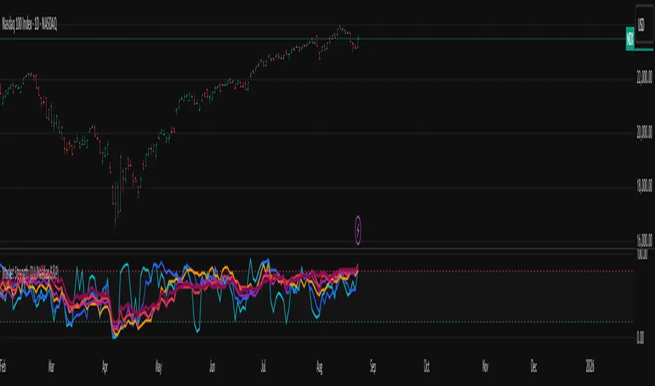
IFVG by Toño# IFVG by Toño - Pine Script Indicator
## Overview
This Pine Script indicator identifies and visualizes **Fair Value Gaps (FVG)** and **Inverted Fair Value Gaps (IFVG)** on trading charts. It provides advanced analysis of price inefficiencies and their subsequent inversions when mitigated.
## Key Features
### 1. Fair Value Gap (FVG) Detection
- **Bullish FVG**: Detected when `low > high ` (gap between current low and high of 2 bars ago)
- **Bearish FVG**: Detected when `high < low ` (gap between current high and low of 2 bars ago)
- Visual representation using colored rectangles (green for bullish, red for bearish)
### 2. Inverted Fair Value Gap (IFVG) Creation
- **IFVG Formation**: When a FVG gets mitigated (price fills the gap with candle body), an IFVG is created
- **Color Inversion**: The IFVG takes the opposite color of the original FVG
- Mitigated bullish FVG → Creates red (bearish) IFVG
- Mitigated bearish FVG → Creates green (bullish) IFVG
- **Mitigation Logic**: Uses only candle body (not wicks) to determine when a FVG is filled
### 3. Customizable Display Options
- **Show Normal FVG**: Toggle visibility of regular Fair Value Gaps
- **Show IFVG**: Toggle visibility of Inverted Fair Value Gaps
- **Smart FVG Display**: Even when "Show Normal FVG" is disabled, FVGs that are part of IFVGs remain visible
- **Extension Control**: Option to extend FVGs until they are mitigated
### 4. IFVG Extension Methods
- **Full Cross Method**: IFVG remains active until price completely crosses through it (including wicks)
- **Number of Bars Method**: IFVG remains active for a specified number of bars (1-100)
### 5. Visual Mitigation Signals
- **Cross Markers**: Shows X-shaped markers when IFVGs are mitigated
- Green cross above bar: Bearish IFVG mitigated
- Red cross below bar: Bullish IFVG mitigated
### 6. Comprehensive Alert System
- **IFVG Formation Alerts**: Notifications when new IFVGs are created
- **IFVG Mitigation Alerts**: Notifications when IFVGs are filled/mitigated
- **Separate Controls**: Individual toggles for bullish and bearish IFVG alerts
## How It Works
### Step-by-Step Process:
1. **FVG Detection**: Script continuously scans for 3-bar patterns that create price gaps
2. **FVG Tracking**: Each FVG is stored with its coordinates, type, and status
3. **Mitigation Monitoring**: Script watches for candle bodies that fill the FVG
4. **IFVG Creation**: Upon mitigation, creates an IFVG with opposite polarity at the same location
5. **IFVG Management**: Tracks and extends IFVGs according to chosen method
6. **Visual Updates**: Dynamically updates colors and visibility based on user settings
## Use Cases
- **Support/Resistance Analysis**: IFVGs often act as strong support/resistance levels
- **Market Structure Understanding**: Helps identify how market inefficiencies get filled and reversed
- **Entry/Exit Timing**: Can be used to time entries around IFVG formations or mitigations
- **Confluence Analysis**: Combine with other technical analysis tools for stronger signals
## Configuration Parameters
- **Colors**: Customizable colors for bullish/bearish FVGs and IFVGs
- **Extension**: Choose how long to display gaps on the chart
- **Alerts**: Full control over notification preferences
- **Visual Clarity**: Options to show/hide different gap types for cleaner charts
## Technical Specifications
- **Pine Script Version**: 5
- **Overlay**: True (displays directly on price chart)
- **Max Boxes**: 500 (supports up to 500 simultaneous gaps)
- **Performance**: Optimized array management for smooth operation
This indicator is particularly valuable for traders who use **Smart Money Concepts (SMC)** and **Inner Circle Trader (ICT)** methodologies, as it provides clear visualization of how institutional order flow creates and fills market inefficiencies.
Elliott Wave - Impulse + Corrective Detector (Demo) เทคนิคการใช้
สำหรับมือใหม่
ดูเฉพาะ Impulse Wave ก่อน
เทรดตาม direction ของ impulse
ใช้ Fibonacci เป็น support/resistance
สำหรับ Advanced
ใช้ Corrective Wave หาจุด reversal
รวม Triangle กับ breakout strategy
ใช้ Complex correction วางแผนระยะยาว
⚙️ การปรับแต่ง
ถ้าเจอ Pattern น้อยเกินไป
ลด Swing Length เป็น 3-4
เพิ่ม Max History เป็น 500
ถ้าเจอ Pattern เยอะเกินไป
เพิ่ม Swing Length เป็น 8-12
ปิด patterns ที่ไม่ต้องการ
สำหรับ Timeframe ต่างๆ
H1-H4: Swing Length = 5-8
Daily: Swing Length = 3-5
Weekly: Swing Length = 2-3
⚠️ ข้อควรระวัง
Elliott Wave เป็น subjective analysis
ใช้ร่วมกับ indicators อื่นๆ
Backtest ก่อนใช้เงินจริง
Pattern อาจเปลี่ยนได้ตลอดเวลา
🎓 สรุป
โค้ดนี้เป็นเครื่องมือช่วยวิเคราะห์ Elliott Wave ที่:
✅ ใช้งานง่าย
✅ ตรวจจับอัตโนมัติ
✅ มี confidence scoring
✅ แสดงผล Fibonacci levels
✅ ส่ง alerts เรียลไทม์
เหมาะสำหรับ: Trader ที่ต้องการใช้ Elliott Wave ในการวิเคราะห์เทคนิค แต่ไม่มีเวลานั่งหา pattern เอง
💡 Usage Tips
For Beginners
Focus on Impulse Waves first
Trade in the direction of impulse
Use Fibonacci as support/resistance levels
For Advanced Users
Use Corrective Waves to find reversal points
Combine Triangles with breakout strategies
Use Complex corrections for long-term planning
⚙️ Customization
If You See Too Few Patterns
Decrease Swing Length to 3-4
Increase Max History to 500
If You See Too Many Patterns
Increase Swing Length to 8-12
Turn off unwanted pattern types
For Different Timeframes
H1-H4: Swing Length = 5-8
Daily: Swing Length = 3-5
Weekly: Swing Length = 2-3
⚠️ Important Warnings
Elliott Wave is subjective analysis
Use with other technical indicators
Backtest before using real money
Patterns can change at any time
🔧 Troubleshooting
No Patterns Showing
Check if you have enough price history
Adjust Swing Length settings
Make sure pattern detection is enabled
Too Many False Signals
Increase confidence threshold requirements
Use higher timeframes
Combine with trend analysis
Performance Issues
Reduce Max History setting
Turn off unnecessary visual elements
Use on liquid markets only
📈 Trading Applications
Entry Strategies
Wave 3 Entry: After Wave 2 completion (61.8%-78.6% retracement)
Wave 5 Target: Equal to Wave 1 or Fibonacci extensions
Corrective Bounce: Trade reversals at C wave completion
Risk Management
Stop Loss: Beyond pattern invalidation levels
Take Profit: Fibonacci extension targets
Position Sizing: Based on pattern confidence
🎓 Summary
This code is an Elliott Wave analysis tool that offers:
✅ Easy to use interface
✅ Automatic pattern detection
✅ Confidence scoring system
✅ Fibonacci level display
✅ Real-time alerts
Perfect for: Traders who want to use Elliott Wave analysis but don't have time to manually identify patterns.
📚 Quick Reference
Pattern Hierarchy (Most to Least Reliable)
Impulse Waves (90% confidence)
Expanded Flats (85% confidence)
Zigzags (80% confidence)
Triangles (75% confidence)
Complex Corrections (70% confidence)
Best Practices
Start with higher timeframes for main trend
Use lower timeframes for precise entries
Always confirm with volume and momentum
Don't trade against strong fundamental news
Keep a trading journal to track performance
Remember: Elliott Wave is an art as much as a science. This tool helps identify potential patterns, but always use your judgment and additional analysis before making trading decisions.
