Tìm kiếm tập lệnh với "Exponential"
Mean-Reversion with CooldownThis strategy requires no indicators or fundamental analysis. It is designed for longer-term positions and works especially well on unleveraged instruments with strong long-term upward trends, such as precious metals. Feel free to experiment with different timeframes — I’ve found that 1-hour charts work particularly well for cryptocurrencies.
The idea is to filter out ongoing bear phases as effectively as possible and capitalize on long-term bull runs.
The script implements an idea that came to me in a state of complete sleep deprivation: open a random long position with a fixed take-profit (TP) and a tight stop-loss (SL).
If the TP is hit — great, we simply try again.
If the SL is triggered — too bad, we pause for a while and then try again.
## Cooldown (Waiting) Mechanism
The waiting mechanism is simple: the more consecutive SL hits we get, the longer we wait before opening the next trade. The waiting time is measured in closed candles, and thus depends on the timeframe you are using.
## Two cooldown calculation modes are currently supported:
### 1. FIBONACCI
The cooldown follows the Fibonacci sequence, based on the number of consecutive losses:
1st loss → wait 1 bar
2nd loss → wait 1 bar
3rd loss → wait 2 or 3 bars (depending on definition)
4th loss → wait 3 or 5 bars
etc.
### 2. POWER OF TWO
The cooldown increases exponentially:
1st loss → wait 2 bars
2nd loss → wait 4 bars
3rd loss → wait 8 bars
4th loss → wait 16 bars
and so on, using the formula 2ⁿ.
## Configurable Parameters
### Cooldown Pause Calculation
The settings allow you to define the SL and TP as percentages of the position value.
The "Cooldown Pause Calculation" option determines how the next cooldown duration is computed after a losing trade.
The system keeps track of how many consecutive losses have occurred since the last profitable trade. That counter is then used to compute how many bars we must wait before opening the next position.
### Maximum Cooldown
The "Max Cooldown Candles" setting defines the maximum number of bars we are allowed to wait before placing a new trade. This prevents the strategy from “locking itself out” for too long and mitigates the fear of missing out (FOMO).
Once the cooldown duration reaches this maximum, the system essentially wraps around and starts the progression again. In the script, this is handled using a simple modulo operation based on the chosen maximum.

Algorithm Predator - ML-liteAlgorithm Predator - ML-lite
This indicator combines four specialized trading agents with an adaptive multi-armed bandit selection system to identify high-probability trade setups. It is designed for swing and intraday traders who want systematic signal generation based on institutional order flow patterns , momentum exhaustion , liquidity dynamics , and statistical mean reversion .
Core Architecture
Why These Components Are Combined:
The script addresses a fundamental challenge in algorithmic trading: no single detection method works consistently across all market conditions. By deploying four independent agents and using reinforcement learning algorithms to select or blend their outputs, the system adapts to changing market regimes without manual intervention.
The Four Trading Agents
1. Spoofing Detector Agent 🎭
Detects iceberg orders through persistent volume at similar price levels over 5 bars
Identifies spoofing patterns via asymmetric wick analysis (wicks exceeding 60% of bar range with volume >1.8× average)
Monitors order clustering using simplified Hawkes process intensity tracking (exponential decay model)
Signal Logic: Contrarian—fades false breakouts caused by institutional manipulation
Best Markets: Consolidations, institutional trading windows, low-liquidity hours
2. Exhaustion Detector Agent ⚡
Calculates RSI divergence between price movement and momentum indicator over 5-bar window
Detects VWAP exhaustion (price at 2σ bands with declining volume)
Uses VPIN reversals (volume-based toxic flow dissipation) to identify momentum failure
Signal Logic: Counter-trend—enters when momentum extreme shows weakness
Best Markets: Trending markets reaching climax points, over-extended moves
3. Liquidity Void Detector Agent 💧
Measures Bollinger Band squeeze (width <60% of 50-period average)
Identifies stop hunts via 20-bar high/low penetration with immediate reversal and volume spike
Detects hidden liquidity absorption (volume >2× average with range <0.3× ATR)
Signal Logic: Breakout anticipation—enters after liquidity grab but before main move
Best Markets: Range-bound pre-breakout, volatility compression zones
4. Mean Reversion Agent 📊
Calculates price z-scores relative to 50-period SMA and standard deviation (triggers at ±2σ)
Implements Ornstein-Uhlenbeck process scoring (mean-reverting stochastic model)
Uses entropy analysis to detect algorithmic trading patterns (low entropy <0.25 = high predictability)
Signal Logic: Statistical reversion—enters when price deviates significantly from statistical equilibrium
Best Markets: Range-bound, low-volatility, algorithmically-dominated instruments
Adaptive Selection: Multi-Armed Bandit System
The script implements four reinforcement learning algorithms to dynamically select or blend agents based on performance:
Thompson Sampling (Default - Recommended):
Uses Bayesian inference with beta distributions (tracks alpha/beta parameters per agent)
Balances exploration (trying underused agents) vs. exploitation (using proven winners)
Each agent's win/loss history informs its selection probability
Lite Approximation: Uses pseudo-random sampling from price/volume noise instead of true random number generation
UCB1 (Upper Confidence Bound):
Calculates confidence intervals using: average_reward + sqrt(2 × ln(total_pulls) / agent_pulls)
Deterministic algorithm favoring agents with high uncertainty (potential upside)
More conservative than Thompson Sampling
Epsilon-Greedy:
Exploits best-performing agent (1-ε)% of the time
Explores randomly ε% of the time (default 10%, configurable 1-50%)
Simple, transparent, easily tuned via epsilon parameter
Gradient Bandit:
Uses softmax probability distribution over agent preference weights
Updates weights via gradient ascent based on rewards
Best for Blend mode where all agents contribute
Selection Modes:
Switch Mode: Uses only the selected agent's signal (clean, decisive)
Blend Mode: Combines all agents using exponentially weighted confidence scores controlled by temperature parameter (smooth, diversified)
Lock Agent Feature:
Optional manual override to force one specific agent
Useful after identifying which agent dominates your specific instrument
Only applies in Switch mode
Four choices: Spoofing Detector, Exhaustion Detector, Liquidity Void, Mean Reversion
Memory System
Dual-Layer Architecture:
Short-Term Memory: Stores last 20 trade outcomes per agent (configurable 10-50)
Long-Term Memory: Stores episode averages when short-term reaches transfer threshold (configurable 5-20 bars)
Memory Boost Mechanism: Recent performance modulates agent scores by up to ±20%
Episode Transfer: When an agent accumulates sufficient results, averages are condensed into long-term storage
Persistence: Manual restoration of learned parameters via input fields (alpha, beta, weights, microstructure thresholds)
How Memory Works:
Agent generates signal → outcome tracked after 8 bars (performance horizon)
Result stored in short-term memory (win = 1.0, loss = 0.0)
Short-term average influences agent's future scores (positive feedback loop)
After threshold met (default 10 results), episode averaged into long-term storage
Long-term patterns (weighted 30%) + short-term patterns (weighted 70%) = total memory boost
Market Microstructure Analysis
These advanced metrics quantify institutional order flow dynamics:
Order Flow Toxicity (Simplified VPIN):
Measures buy/sell volume imbalance over 20 bars: |buy_vol - sell_vol| / (buy_vol + sell_vol)
Detects informed trading activity (institutional players with non-public information)
Values >0.4 indicate "toxic flow" (informed traders active)
Lite Approximation: Uses simple open/close heuristic instead of tick-by-tick trade classification
Price Impact Analysis (Simplified Kyle's Lambda):
Measures market impact efficiency: |price_change_10| / sqrt(volume_sum_10)
Low values = large orders with minimal price impact ( stealth accumulation )
High values = retail-dominated moves with high slippage
Lite Approximation: Uses simplified denominator instead of regression-based signed order flow
Market Randomness (Entropy Analysis):
Counts unique price changes over 20 bars / 20
Measures market predictability
High entropy (>0.6) = human-driven, chaotic price action
Low entropy (<0.25) = algorithmic trading dominance (predictable patterns)
Lite Approximation: Simple ratio instead of true Shannon entropy H(X) = -Σ p(x)·log₂(p(x))
Order Clustering (Simplified Hawkes Process):
Tracks self-exciting event intensity (coordinated order activity)
Decays at 0.9× per bar, spikes +1.0 when volume >1.5× average
High intensity (>0.7) indicates clustering (potential spoofing/accumulation)
Lite Approximation: Simple exponential decay instead of full λ(t) = μ + Σ α·exp(-β(t-tᵢ)) with MLE
Signal Generation Process
Multi-Stage Validation:
Stage 1: Agent Scoring
Each agent calculates internal score based on its detection criteria
Scores must exceed agent-specific threshold (adjusted by sensitivity multiplier)
Agent outputs: Signal direction (+1/-1/0) and Confidence level (0.0-1.0)
Stage 2: Memory Boost
Agent scores multiplied by memory boost factor (0.8-1.2 based on recent performance)
Successful agents get amplified, failing agents get dampened
Stage 3: Bandit Selection/Blending
If Adaptive Mode ON:
Switch: Bandit selects single best agent, uses only its signal
Blend: All agents combined using softmax-weighted confidence scores
If Adaptive Mode OFF:
Traditional consensus voting with confidence-squared weighting
Signal fires when consensus exceeds threshold (default 70%)
Stage 4: Confirmation Filter
Raw signal must repeat for consecutive bars (default 3, configurable 2-4)
Minimum confidence threshold: 0.25 (25%) enforced regardless of mode
Trend alignment check: Long signals require trend_score ≥ -2, Short signals require trend_score ≤ 2
Stage 5: Cooldown Enforcement
Minimum bars between signals (default 10, configurable 5-15)
Prevents over-trading during choppy conditions
Stage 6: Performance Tracking
After 8 bars (performance horizon), signal outcome evaluated
Win = price moved in signal direction, Loss = price moved against
Results fed back into memory and bandit statistics
Trading Modes (Presets)
Pre-configured parameter sets:
Conservative: 85% consensus, 4 confirmations, 15-bar cooldown
Expected: 60-70% win rate, 3-8 signals/week
Best for: Swing trading, capital preservation, beginners
Balanced: 70% consensus, 3 confirmations, 10-bar cooldown
Expected: 55-65% win rate, 8-15 signals/week
Best for: Day trading, most traders, general use
Aggressive: 60% consensus, 2 confirmations, 5-bar cooldown
Expected: 50-58% win rate, 15-30 signals/week
Best for: Scalping, high-frequency trading, active management
Elite: 75% consensus, 3 confirmations, 12-bar cooldown
Expected: 58-68% win rate, 5-12 signals/week
Best for: Selective trading, high-conviction setups
Adaptive: 65% consensus, 2 confirmations, 8-bar cooldown
Expected: Varies based on learning
Best for: Experienced users leveraging bandit system
How to Use
1. Initial Setup (5 Minutes):
Select Trading Mode matching your style (start with Balanced)
Enable Adaptive Learning (recommended for automatic agent selection)
Choose Thompson Sampling algorithm (best all-around performance)
Keep Microstructure Metrics enabled for liquid instruments (>100k daily volume)
2. Agent Tuning (Optional):
Adjust Agent Sensitivity multipliers (0.5-2.0):
<0.8 = Highly selective (fewer signals, higher quality)
0.9-1.2 = Balanced (recommended starting point)
1.3 = Aggressive (more signals, lower individual quality)
Monitor dashboard for 20-30 signals to identify dominant agent
If one agent consistently outperforms, consider using Lock Agent feature
3. Bandit Configuration (Advanced):
Blend Temperature (0.1-2.0):
0.3 = Sharp decisions (best agent dominates)
0.5 = Balanced (default)
1.0+ = Smooth (equal weighting, democratic)
Memory Decay (0.8-0.99):
0.90 = Fast adaptation (volatile markets)
0.95 = Balanced (most instruments)
0.97+ = Long memory (stable trends)
4. Signal Interpretation:
Green triangle (▲): Long signal confirmed
Red triangle (▼): Short signal confirmed
Dashboard shows:
Active agent (highlighted row with ► marker)
Win rate per agent (green >60%, yellow 40-60%, red <40%)
Confidence bars (█████ = maximum confidence)
Memory size (short-term buffer count)
Colored zones display:
Entry level (current close)
Stop-loss (1.5× ATR)
Take-profit 1 (2.0× ATR)
Take-profit 2 (3.5× ATR)
5. Risk Management:
Never risk >1-2% per signal (use ATR-based stops)
Signals are entry triggers, not complete strategies
Combine with your own market context analysis
Consider fundamental catalysts and news events
Use "Confirming" status to prepare entries (not to enter early)
6. Memory Persistence (Optional):
After 50-100 trades, check Memory Export Panel
Record displayed alpha/beta/weight values for each agent
Record VPIN and Kyle threshold values
Enable "Restore From Memory" and input saved values to continue learning
Useful when switching timeframes or restarting indicator
Visual Components
On-Chart Elements:
Spectral Layers: EMA8 ± 0.5 ATR bands (dynamic support/resistance, colored by trend)
Energy Radiance: Multi-layer glow boxes at signal points (intensity scales with confidence, configurable 1-5 layers)
Probability Cones: Projected price paths with uncertainty wedges (15-bar projection, width = confidence × ATR)
Connection Lines: Links sequential signals (solid = same direction continuation, dotted = reversal)
Kill Zones: Risk/reward boxes showing entry, stop-loss, and dual take-profit targets
Signal Markers: Triangle up/down at validated entry points
Dashboard (Configurable Position & Size):
Regime Indicator: 4-level trend classification (Strong Bull/Bear, Weak Bull/Bear)
Mode Status: Shows active system (Adaptive Blend, Locked Agent, or Consensus)
Agent Performance Table: Real-time win%, confidence, and memory stats
Order Flow Metrics: Toxicity and impact indicators (when microstructure enabled)
Signal Status: Current state (Long/Short/Confirming/Waiting) with confirmation progress
Memory Panel (Configurable Position & Size):
Live Parameter Export: Alpha, beta, and weight values per agent
Adaptive Thresholds: Current VPIN sensitivity and Kyle threshold
Save Reminder: Visual indicator if parameters should be recorded
What Makes This Original
This script's originality lies in three key innovations:
1. Genuine Meta-Learning Framework:
Unlike traditional indicator mashups that simply display multiple signals, this implements authentic reinforcement learning (multi-armed bandits) to learn which detection method works best in current conditions. The Thompson Sampling implementation with beta distribution tracking (alpha for successes, beta for failures) is statistically rigorous and adapts continuously. This is not post-hoc optimization—it's real-time learning.
2. Episodic Memory Architecture with Transfer Learning:
The dual-layer memory system mimics human learning patterns:
Short-term memory captures recent performance (recency bias)
Long-term memory preserves historical patterns (experience)
Automatic transfer mechanism consolidates knowledge
Memory boost creates positive feedback loops (successful strategies become stronger)
This architecture allows the system to adapt without retraining , unlike static ML models that require batch updates.
3. Institutional Microstructure Integration:
Combines retail-focused technical analysis (RSI, Bollinger Bands, VWAP) with institutional-grade microstructure metrics (VPIN, Kyle's Lambda, Hawkes processes) typically found in academic finance literature and professional trading systems, not standard retail platforms. While simplified for Pine Script constraints, these metrics provide insight into informed vs. uninformed trading , a dimension entirely absent from traditional technical analysis.
Mashup Justification:
The four agents are combined specifically for risk diversification across failure modes:
Spoofing Detector: Prevents false breakout losses from manipulation
Exhaustion Detector: Prevents chasing extended trends into reversals
Liquidity Void: Exploits volatility compression (different regime than trending)
Mean Reversion: Provides mathematical anchoring when patterns fail
The bandit system ensures the optimal tool is automatically selected for each market situation, rather than requiring manual interpretation of conflicting signals.
Why "ML-lite"? Simplifications and Approximations
This is the "lite" version due to necessary simplifications for Pine Script execution:
1. Simplified VPIN Calculation:
Academic Implementation: True VPIN uses volume bucketing (fixed-volume bars) and tick-by-tick buy/sell classification via Lee-Ready algorithm or exchange-provided trade direction flags
This Implementation: 20-bar rolling window with simple open/close heuristic (close > open = buy volume)
Impact: May misclassify volume during ranging/choppy markets; works best in directional moves
2. Pseudo-Random Sampling:
Academic Implementation: Thompson Sampling requires true random number generation from beta distributions using inverse transform sampling or acceptance-rejection methods
This Implementation: Deterministic pseudo-randomness derived from price and volume decimal digits: (close × 100 - floor(close × 100)) + (volume % 100) / 100
Impact: Not cryptographically random; may have subtle biases in specific price ranges; provides sufficient variation for agent selection
3. Hawkes Process Approximation:
Academic Implementation: Full Hawkes process uses maximum likelihood estimation with exponential kernels: λ(t) = μ + Σ α·exp(-β(t-tᵢ)) fitted via iterative optimization
This Implementation: Simple exponential decay (0.9 multiplier) with binary event triggers (volume spike = event)
Impact: Captures self-exciting property but lacks parameter optimization; fixed decay rate may not suit all instruments
4. Kyle's Lambda Simplification:
Academic Implementation: Estimated via regression of price impact on signed order flow over multiple time intervals: Δp = λ × Δv + ε
This Implementation: Simplified ratio: price_change / sqrt(volume_sum) without proper signed order flow or regression
Impact: Provides directional indicator of impact but not true market depth measurement; no statistical confidence intervals
5. Entropy Calculation:
Academic Implementation: True Shannon entropy requires probability distribution: H(X) = -Σ p(x)·log₂(p(x)) where p(x) is probability of each price change magnitude
This Implementation: Simple ratio of unique price changes to total observations (variety measure)
Impact: Measures diversity but not true information entropy with probability weighting; less sensitive to distribution shape
6. Memory System Constraints:
Full ML Implementation: Neural networks with backpropagation, experience replay buffers (storing state-action-reward tuples), gradient descent optimization, and eligibility traces
This Implementation: Fixed-size array queues with simple averaging; no gradient-based learning, no state representation beyond raw scores
Impact: Cannot learn complex non-linear patterns; limited to linear performance tracking
7. Limited Feature Engineering:
Advanced Implementation: Dozens of engineered features, polynomial interactions (x², x³), dimensionality reduction (PCA, autoencoders), feature selection algorithms
This Implementation: Raw agent scores and basic market metrics (RSI, ATR, volume ratio); minimal transformation
Impact: May miss subtle cross-feature interactions; relies on agent-level intelligence rather than feature combinations
8. Single-Instrument Data:
Full Implementation: Multi-asset correlation analysis (sector ETFs, currency pairs, volatility indices like VIX), lead-lag relationships, risk-on/risk-off regimes
This Implementation: Only OHLCV data from displayed instrument
Impact: Cannot incorporate broader market context; vulnerable to correlated moves across assets
9. Fixed Performance Horizon:
Full Implementation: Adaptive horizon based on trade duration, volatility regime, or profit target achievement
This Implementation: Fixed 8-bar evaluation window
Impact: May evaluate too early in slow markets or too late in fast markets; one-size-fits-all approach
Performance Impact Summary:
These simplifications make the script:
✅ Faster: Executes in milliseconds vs. seconds (or minutes) for full academic implementations
✅ More Accessible: Runs on any TradingView plan without external data feeds, APIs, or compute servers
✅ More Transparent: All calculations visible in Pine Script (no black-box compiled models)
✅ Lower Resource Usage: <500 bars lookback, minimal memory footprint
⚠️ Less Precise: Approximations may reduce statistical edge by 5-15% vs. academic implementations
⚠️ Limited Scope: Cannot capture tick-level dynamics, multi-order-book interactions, or cross-asset flows
⚠️ Fixed Parameters: Some thresholds hardcoded rather than dynamically optimized
When to Upgrade to Full Implementation:
Consider professional Python/C++ versions with institutional data feeds if:
Trading with >$100K capital where precision differences materially impact returns
Operating in microsecond-competitive environments (HFT, market making)
Requiring regulatory-grade audit trails and reproducibility
Backtesting with tick-level precision for strategy validation
Need true real-time adaptation with neural network-based learning
For retail swing/day trading and position management, these approximations provide sufficient signal quality while maintaining usability, transparency, and accessibility. The core logic—multi-agent detection with adaptive selection—remains intact.
Technical Notes
All calculations use standard Pine Script built-in functions ( ta.ema, ta.atr, ta.rsi, ta.bb, ta.sma, ta.stdev, ta.vwap )
VPIN and Kyle's Lambda use simplified formulas optimized for OHLCV data (see "Lite" section above)
Thompson Sampling uses pseudo-random noise from price/volume decimal digits for beta distribution sampling
No repainting: All calculations use confirmed bar data (no forward-looking)
Maximum lookback: 500 bars (set via max_bars_back parameter)
Performance evaluation: 8-bar forward-looking window for reward calculation (clearly disclosed)
Confidence threshold: Minimum 0.25 (25%) enforced on all signals
Memory arrays: Dynamic sizing with FIFO queue management
Limitations and Disclaimers
Not Predictive: This indicator identifies patterns in historical data. It cannot predict future price movements with certainty.
Requires Human Judgment: Signals are entry triggers, not complete trading strategies. Must be confirmed with your own analysis, risk management rules, and market context.
Learning Period Required: The adaptive system requires 50-100 bars minimum to build statistically meaningful performance data for bandit algorithms.
Overfitting Risk: Restoring memory parameters from one market regime to a drastically different regime (e.g., low volatility to high volatility) may cause poor initial performance until system re-adapts.
Approximation Limitations: Simplified calculations (see "Lite" section) may underperform academic implementations by 5-15% in highly efficient markets.
No Guarantee of Profit: Past performance, whether backtested or live-traded, does not guarantee future performance. All trading involves risk of loss.
Forward-Looking Bias: Performance evaluation uses 8-bar forward window—this creates slight look-ahead for learning (though not for signals). Real-time performance may differ from indicator's internal statistics.
Single-Instrument Limitation: Does not account for correlations with related assets or broader market regime changes.
Recommended Settings
Timeframe: 15-minute to 4-hour charts (sufficient volatility for ATR-based stops; adequate bar volume for learning)
Assets: Liquid instruments with >100k daily volume (forex majors, large-cap stocks, BTC/ETH, major indices)
Not Recommended: Illiquid small-caps, penny stocks, low-volume altcoins (microstructure metrics unreliable)
Complementary Tools: Volume profile, order book depth, market breadth indicators, fundamental catalysts
Position Sizing: Risk no more than 1-2% of capital per signal using ATR-based stop-loss
Signal Filtering: Consider external confluence (support/resistance, trendlines, round numbers, session opens)
Start With: Balanced mode, Thompson Sampling, Blend mode, default agent sensitivities (1.0)
After 30+ Signals: Review agent win rates, consider increasing sensitivity of top performers or locking to dominant agent
Alert Configuration
The script includes built-in alert conditions:
Long Signal: Fires when validated long entry confirmed
Short Signal: Fires when validated short entry confirmed
Alerts fire once per bar (after confirmation requirements met)
Set alert to "Once Per Bar Close" for reliability
Taking you to school. — Dskyz, Trade with insight. Trade with anticipation.

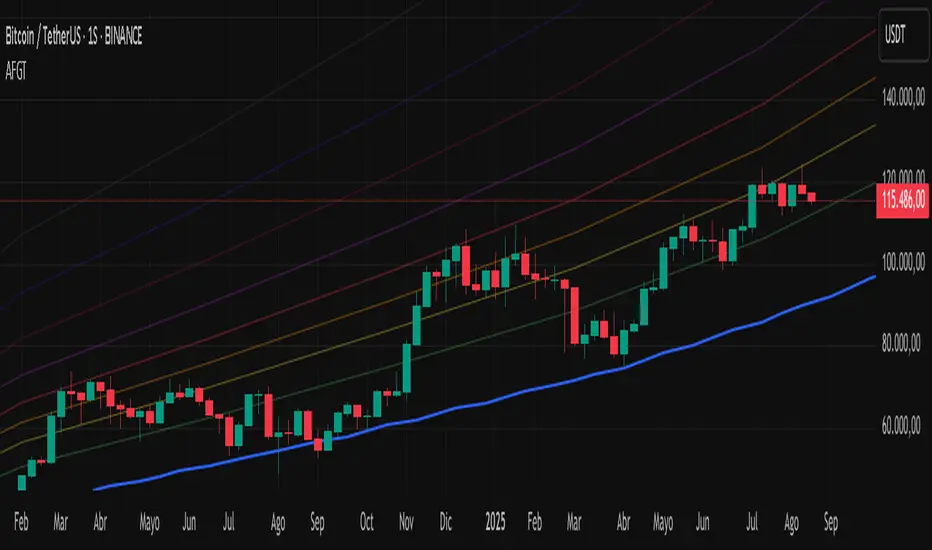
Auto-Fit Growth Trendline# **Theoretical Algorithmic Principles of the Auto-Fit Growth Trendline (AFGT)**
## **🎯 What Does This Algorithm Do?**
The Auto-Fit Growth Trendline is an advanced technical analysis system that **automates the identification of long-term growth trends** and **projects future price levels** based on historical cyclical patterns.
### **Primary Functionality:**
- **Automatically detects** the most significant lows in regular periods (monthly, quarterly, semi-annually, annually)
- **Constructs a dynamic trendline** that connects these historical lows
- **Projects the trend into the future** with high mathematical precision
- **Generates Fibonacci bands** that act as dynamic support and resistance levels
- **Automatically adapts** to different timeframes and market conditions
### **Strategic Purpose:**
The algorithm is designed to identify **fundamental value zones** where price has historically found support, enabling traders to:
- Identify optimal entry points for long positions
- Establish realistic price targets based on mathematical projections
- Recognize dynamic support and resistance levels
- Anticipate long-term price movements
---
## **🧮 Core Mathematical Foundations**
### **Adaptive Temporal Segmentation Theory**
The algorithm is based on **dynamic temporal partition theory**, where time is divided into mathematically coherent uniform intervals. It uses modular transformations to create bijective mappings between continuous timestamps and discrete periods, ensuring each temporal point belongs uniquely to a specific period.
**What does this achieve?** It allows the algorithm to automatically identify natural market cycles (annual, quarterly, etc.) without manual intervention, adapting to the inherent periodicity of each asset.
The temporal mapping function implements a **discrete affine transformation** that normalizes different frequencies (monthly, quarterly, semi-annual, annual) to a space of unique identifiers, enabling consistent cross-temporal comparative analysis.
---
## **📊 Local Extrema Detection Theory**
### **Multi-Point Retrospective Validation Principle**
Local minima detection is founded on **relative extrema theory with sliding window**. Instead of using a simple minimum finder, it implements a cross-validation system that examines the persistence of the extremum across multiple historical periods.
**What problem does this solve?** It eliminates false minima caused by temporal volatility, identifying only those points that represent true historical support levels with statistical significance.
This approach is based on the **statistical confirmation principle**, where a minimum is only considered valid if it maintains its extremum condition during a defined observation period, significantly reducing false positives caused by transitory volatility.
---
## **🔬 Robust Interpolation Theory with Outlier Control**
### **Contextual Adaptive Interpolation Model**
The mathematical core uses **piecewise linear interpolation with adaptive outlier correction**. The key innovation lies in implementing a **contextual anomaly detector** that identifies not only absolute extreme values, but relative deviations to the local context.
**Why is this important?** Financial markets contain extreme events (crashes, bubbles) that can distort projections. This system identifies and appropriately weights them without completely eliminating them, preserving directional information while attenuating distortions.
### **Implicit Bayesian Smoothing Algorithm**
When an outlier is detected (deviation >300% of local average), the system applies a **simplified Kalman filter** that combines the current observation with a local trend estimation, using a weight factor that preserves directional information while attenuating extreme fluctuations.
---
## **📈 Stabilized Extrapolation Theory**
### **Exponential Growth Model with Dampening**
Extrapolation is based on a **modified exponential growth model with progressive dampening**. It uses multiple historical points to calculate local growth ratios, implements statistical filtering to eliminate outliers, and applies a dampening factor that increases with extrapolation distance.
**What advantage does this offer?** Long-term projections in finance tend to be exponentially unrealistic. This system maintains short-to-medium term accuracy while converging toward realistic long-term projections, avoiding the typical "exponential explosions" of other methods.
### **Asymptotic Convergence Principle**
For long-term projections, the algorithm implements **controlled asymptotic convergence**, where growth ratios gradually converge toward pre-established limits, avoiding unrealistic exponential projections while preserving short-to-medium term accuracy.
---
## **🌟 Dynamic Fibonacci Projection Theory**
### **Continuous Proportional Scaling Model**
Fibonacci bands are constructed through **uniform proportional scaling** of the base curve, where each level represents a linear transformation of the main curve by a constant factor derived from the Fibonacci sequence.
**What is its practical utility?** It provides dynamic resistance and support levels that move with the trend, offering price targets and profit-taking points that automatically adapt to market evolution.
### **Topological Preservation Principle**
The system maintains the **topological properties** of the base curve in all Fibonacci projections, ensuring that spatial and temporal relationships are consistently preserved across all resistance/support levels.
---
## **⚡ Adaptive Computational Optimization**
### **Multi-Scale Resolution Theory**
It implements **automatic multi-resolution analysis** where data granularity is dynamically adjusted according to the analysis timeframe. It uses the **adaptive Nyquist principle** to optimize the signal-to-noise ratio according to the temporal observation scale.
**Why is this necessary?** Different timeframes require different levels of detail. A 1-minute chart needs more granularity than a monthly one. This system automatically optimizes resolution for each case.
### **Adaptive Density Algorithm**
Calculation point density is optimized through **adaptive sampling theory**, where calculation frequency is adjusted according to local trend curvature and analysis timeframe, balancing visual precision with computational efficiency.
---
## **🛡️ Robustness and Fault Tolerance**
### **Graceful Degradation Theory**
The system implements **multi-level graceful degradation**, where under error conditions or insufficient data, the algorithm progressively falls back to simpler but reliable methods, maintaining basic functionality under any condition.
**What does this guarantee?** That the indicator functions consistently even with incomplete data, new symbols with limited history, or extreme market conditions.
### **State Consistency Principle**
It uses **mathematical invariants** to guarantee that the algorithm's internal state remains consistent between executions, implementing consistency checks that validate data structure integrity in each iteration.
---
## **🔍 Key Theoretical Innovations**
### **A. Contextual vs. Absolute Outlier Detection**
It revolutionizes traditional outlier detection by considering not only the absolute magnitude of deviations, but their relative significance within the local context of the time series.
**Practical impact:** It distinguishes between legitimate market movements and technical anomalies, preserving important events like breakouts while filtering noise.
### **B. Extrapolation with Weighted Historical Memory**
It implements a memory system that weights different historical periods according to their relevance for current prediction, creating projections more adaptable to market regime changes.
**Competitive advantage:** It automatically adapts to fundamental changes in asset dynamics without requiring manual recalibration.
### **C. Automatic Multi-Timeframe Adaptation**
It develops an automatic temporal resolution selection system that optimizes signal extraction according to the intrinsic characteristics of the analysis timeframe.
**Result:** A single indicator that functions optimally from 1-minute to monthly charts without manual adjustments.
### **D. Intelligent Asymptotic Convergence**
It introduces the concept of controlled asymptotic convergence in financial extrapolations, where long-term projections converge toward realistic limits based on historical fundamentals.
**Added value:** Mathematically sound long-term projections that avoid the unrealistic extremes typical of other extrapolation methods.
---
## **📊 Complexity and Scalability Theory**
### **Optimized Linear Complexity Model**
The algorithm maintains **linear computational complexity** O(n) in the number of historical data points, guaranteeing scalability for extensive time series analysis without performance degradation.
### **Temporal Locality Principle**
It implements **temporal locality**, where the most expensive operations are concentrated in the most relevant temporal regions (recent periods and near projections), optimizing computational resource usage.
---
## **🎯 Convergence and Stability**
### **Probabilistic Convergence Theory**
The system guarantees **probabilistic convergence** toward the real underlying trend, where projection accuracy increases with the amount of available historical data, following **law of large numbers** principles.
**Practical implication:** The more history an asset has, the more accurate the algorithm's projections will be.
### **Guaranteed Numerical Stability**
It implements **intrinsic numerical stability** through the use of robust floating-point arithmetic and validations that prevent overflow, underflow, and numerical error propagation.
**Result:** Reliable operation even with extreme-priced assets (from satoshis to thousand-dollar stocks).
---
## **💼 Comprehensive Practical Application**
**The algorithm functions as a "financial GPS"** that:
1. **Identifies where we've been** (significant historical lows)
2. **Determines where we are** (current position relative to the trend)
3. **Projects where we're going** (future trend with specific price levels)
4. **Provides alternative routes** (Fibonacci bands as alternative targets)
This theoretical framework represents an innovative synthesis of time series analysis, approximation theory, and computational optimization, specifically designed for long-term financial trend analysis with robust and mathematically grounded projections.
remaLibrary " REMA "
Custom Regional Exponential Moving Average with enhanced sensitivity to recent price action
Description: What Makes REMA Unique?
REMA introduces a dual-region weighting system that intelligently balances short-term responsiveness with long-term trend context, solving the fundamental limitation of standard EMAs where longer periods necessarily sacrifice recent price sensitivity.
Key Differences from Standard EMA:
Adaptive Regional Weighting: Applies stronger exponential decay to recent price data while maintaining appropriate weighting for historical context.
Maintains Responsiveness at Any Length: Unlike standard EMAs where longer periods become progressively less responsive, REMA preserves significant sensitivity to recent price action even at 100+ period lengths.
Mathematically Sound Enhancement: Preserves the core mathematical integrity of exponential averaging while introducing region-specific weighting that better reflects how traders actually interpret price action.
Value to TradingView Community:
Improved Signal Timing: Detects reversals 1-3 bars earlier than traditional EMAs without increasing false signals.
Better Multi-Timeframe Analysis: Provides more consistent behavior across different period settings, reducing conflicting signals between timeframes.
Ideal for Modern Markets: Better handles today's high-volatility, algorithm-driven markets where traditional indicators often lag too much to be effective.
Optimized for Both Trend and Reversal Trading: Simultaneously provides strong trend-following capabilities while remaining sensitive to legitimate reversal signals.
Computation Efficiency: The fast implementation offers enhanced capabilities with minimal computational overhead, making it practical for real-time analysis.
REMA fills a critical gap between lagging long-period EMAs and noisy short-period EMAs, giving traders a single, versatile tool that adapts to market conditions more effectively than standard technical indicators.
Implementation:
rema(src, length, recency_bias, transition_point)
Regional Exponential Moving Average that maintains recent price sensitivity even with long lookback periods
Parameters:
src (float) : Input source series
length (int) : Overall EMA period length
recency_bias (float) : Weighting factor to increase sensitivity to recent prices (1.0-3.0 recommended)
transition_point (float) : Percentage point (0.0-1.0) in the lookback period where weighting shifts from recent to historical
Returns: Custom exponentially weighted moving average with regional bias
rema_fast(src, length, recency_bias)
Simplified Regional EMA that uses a recursive calculation method
Parameters:
src (float) : Input source series
length (int) : Overall EMA period
recency_bias (float) : Factor to increase sensitivity to recent price (1.0-3.0 recommended)
Returns: Computationally efficient regional EMA
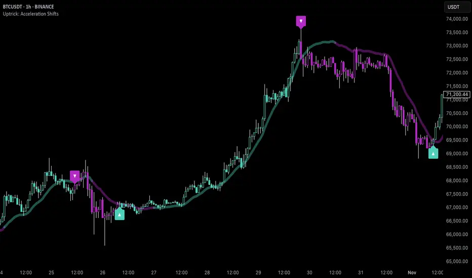
Uptrick: Acceleration ShiftsIntroduction
Uptrick: Acceleration Shifts is designed to measure and visualize price momentum shifts by focusing on acceleration —the rate of change in velocity over time. It uses various moving average techniques as a trend filter, providing traders with a clearer perspective on market direction and potential trade entries or exits.
Purpose
The main goal of this indicator is to spot strong momentum changes (accelerations) and confirm them with a chosen trend filter. It attempts to distinguish genuine market moves from noise, helping traders make more informed decisions. The script can also trigger multiple entries (smart pyramiding) within the same trend, if desired.
Overview
By measuring how quickly price velocity changes (acceleration) and comparing it against a smoothed average of itself, this script generates buy or sell signals once the acceleration surpasses a given threshold. A trend filter is added for further validation. Users can choose from multiple smoothing methods and color schemes, and they can optionally enable a small table that displays real-time acceleration values.
Originality and Uniqueness
This script offers an acceleration-based approach, backed by several different moving average choices. The blend of acceleration thresholds, a trend filter, and an optional extra-entry (pyramiding) feature provides a flexible toolkit for various trading styles. The inclusion of multiple color themes and a slope-based coloring of the trend line adds clarity and user customization.
Inputs & Features
1. Acceleration Length (length)
This input determines the number of bars used when calculating velocity. Specifically, the script computes velocity by taking the difference in closing prices over length bars, and then calculates acceleration based on how that velocity changes over an additional length. The default is 14.
2. Trend Filter Length (smoothing)
This sets the lookback period for the chosen trend filter method. The default of 50 results in a moderately smooth trend line. A higher smoothing value will create a slower-moving trend filter.
3. Acceleration Threshold (threshold)
This multiplier determines when acceleration is considered strong enough to trigger a main buy or sell signal. A default value of 2.5 means the current acceleration must exceed 2.5 times the average acceleration before signaling.
4. Smart Pyramiding Strength (pyramidingThreshold)
This lower threshold is used for additional (pyramiding) entries once the main trend has already been identified. For instance, if set to 0.5, the script looks for acceleration crossing ±0.5 times its average acceleration to add extra positions.
5. Max Pyramiding Entries (maxPyramidingEntries)
This sets a limit on how many extra positions can be opened (beyond the first main signal) in a single directional trend. The default of 3 ensures traders do not become overexposed.
6. Show Acceleration Table (showTable)
When enabled, a small table displaying the current acceleration and its average is added to the top-right corner of the chart. This table helps monitor real-time momentum changes.
7. Smart Pyramiding (enablePyramiding)
This toggle decides whether additional entries (buy or sell) will be generated once a main signal is active. If enabled, these extra signals act as filtered entries, only firing when acceleration re-crosses a smaller threshold (pyramidingThreshold). These signals have a '+' next to their signal on the label.
8. Select Color Scheme (selectedColorScheme)
Allows choosing between various pre-coded color themes, such as Default, Emerald, Sapphire, Golden Blaze, Mystic, Monochrome, Pastel, Vibrant, Earth, or Neon. Each theme applies a distinct pair of colors for bullish and bearish conditions.
9. Trend Filter (TrendFilter)
Lets the user pick one of several moving average approaches to determine the prevailing trend. The options include:
Short Term (TEMA)
EWMA
Medium Term (HMA)
Classic (SMA)
Quick Reaction (DEMA)
Each method behaves differently, balancing reactivity and smoothness.
10. Slope Lookback (slopeOffset)
Used to measure the slope of the trend filter over a set number of bars (default is 10). This slope then influences the coloring of the trend filter line, indicating bullish or bearish tilt.
Note: The script refers to this as the "Massive Slope Index," but it effectively serves as a Trend Slope Calculation, measuring how the chosen trend filter changes over a specified period.
11. Alerts for Buy/Sell and Pyramiding Signals
The script includes built-in alert conditions that can be enabled or configured. These alerts trigger whenever the script detects a main Buy or Sell signal, as well as extra (pyramiding) signals if Smart Pyramiding is active. This feature allows traders to receive immediate notifications or automate a trading response.
Calculation Methodology
1. Velocity and Acceleration
Velocity is derived by subtracting the closing price from its value length bars ago. Acceleration is the difference in velocity over an additional length period. This highlights how quickly momentum is shifting.
2. Average Acceleration
The script smooths raw acceleration with a simple moving average (SMA) using the smoothing input. Comparing current acceleration against this average provides a threshold-based signal mechanism.
3. Trend Filter
Users can pick one of five moving average types to form a trend baseline. These range from quick-reacting methods (DEMA, TEMA) to smoother options (SMA, HMA, EWMA). The script checks whether the price is above or below this filter to confirm trend direction.
4. Buy/Sell Logic
A buy occurs when acceleration surpasses avgAcceleration * threshold and price closes above the trend filter. A sell occurs under the opposite conditions. An additional overbought/oversold check (based on a longer SMA) refines these signals further.
When price is considered oversold (i.e., close is below a longer-term SMA), a bullish acceleration signal has a higher likelihood of success because it indicates that the market is attempting to reverse from a lower price region. Conversely, when price is considered overbought (close is above this longer-term SMA), a bearish acceleration signal is more likely to be valid. This helps reduce false signals by waiting until the market is extended enough that a reversal or continuation has a stronger chance of following through.
5. Smart Pyramiding
Once a main buy or sell signal is triggered, additional (filtered) entries can be taken if acceleration crosses a smaller multiplier (pyramidingThreshold). This helps traders scale into strong moves. The script enforces a cap (maxPyramidingEntries) to limit risk.
6. Visual Elements
Candles can be recolored based on the active signal. Labels appear on the chart whenever a main or pyramiding entry signal is triggered. An optional table can show real-time acceleration values.
Color Schemes
The script includes a variety of predefined color themes. For bullish conditions, it might use turquoise or green, and for bearish conditions, magenta or red—depending on which color scheme the user selects. Each scheme aims to provide clear visual differentiation between bullish and bearish market states.
Why Each Indicator Was Part of This Component
Acceleration is employed to detect swift changes in momentum, capturing shifts that may not yet appear in more traditional measures. To further adapt to different trading styles and market conditions, several moving average methods are incorporated:
• TEMA (Triple Exponential Moving Average) is chosen for its ability to reduce lag more effectively than a standard EMA while still reacting swiftly to price changes. Its construction layers exponential smoothing in a way that can highlight sudden momentum shifts without sacrificing too much smoothness.
• DEMA (Double Exponential Moving Average) provides a faster response than a single EMA by using two layers of exponential smoothing. It is slightly less smoothed than TEMA but can alert traders to momentum changes earlier, though with a higher risk of noise in choppier markets.
• HMA (Hull Moving Average) is known for its balance of smoothness and reduced lag. Its weighted calculations help track trend direction clearly, making it useful for traders who want a smoother line that still reacts fairly quickly.
• SMA (Simple Moving Average) is the classic baseline for smoothing price data. It offers a clear, stable perspective on long-term trends, though it reacts more slowly than other methods. Its simplicity can be beneficial in lower-volatility or more stable market environments.
• EWMA (Exponentially Weighted Moving Average) provides a middle ground by emphasizing recent price data while still retaining some degree of smoothing. It typically responds faster than an SMA but is less aggressive than DEMA or TEMA.
Alongside these moving average techniques, the script employs a slope calculation (referred to as the “Massive Slope Index”) to visually indicate whether the chosen filter is sloping upward or downward. This adds an extra layer of clarity to directional analysis. The indicator also uses overbought/oversold checks, based on a longer-term SMA, to help filter out signals in overstretched markets—reducing the likelihood of false entries in conditions where the price is already extensively extended.
Additional Features
Alerts can be set up for both main signals and additional pyramiding signals, which is helpful for automated or semi-automated trading. The optional acceleration table offers quick reference values, making momentum monitoring more intuitive. Including explicit alert conditions for Buy/Sell and Pyramiding ensures traders can respond promptly to market movements or integrate these triggers into automated strategies.
Summary
This script serves as a comprehensive momentum-based trading framework, leveraging acceleration metrics and multiple moving average filters to identify potential shifts in market direction. By combining overbought/oversold checks with threshold-based triggers, it aims to reduce the noise that commonly plagues purely reactive indicators. The flexibility of Smart Pyramiding, customizable color schemes, and built-in alerts allows users to tailor their experience and respond swiftly to valid signals, potentially enhancing trading decisions across various market conditions.
Disclaimer
All trading involves significant risk, and users should apply their own judgment, risk management, and broader analysis before making investment decisions.
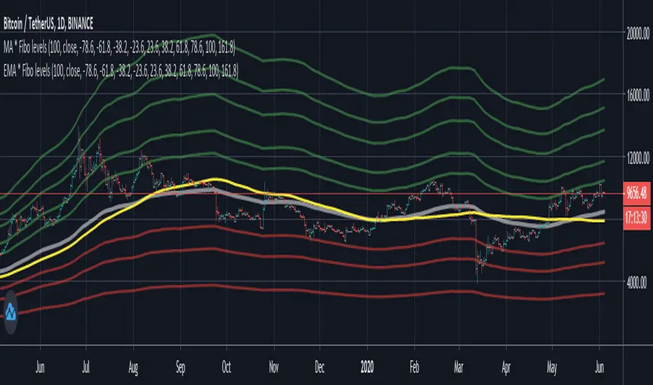
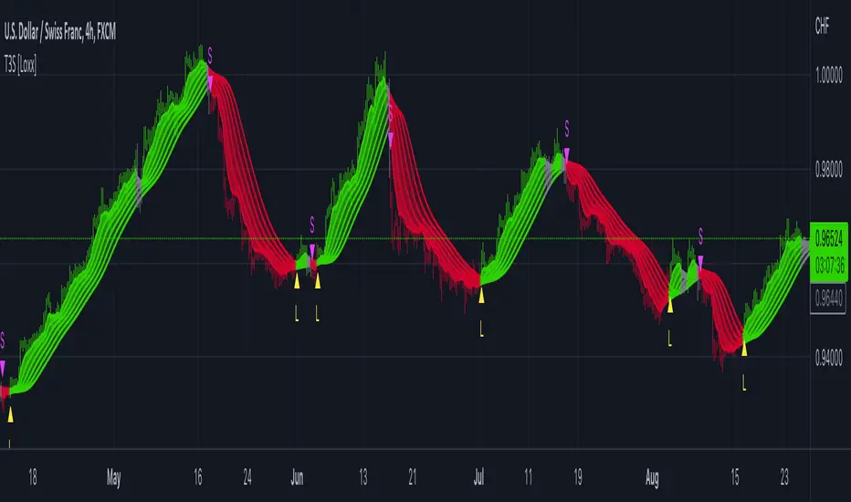
STD-Adaptive T3 [Loxx]STD-Adaptive T3 is a standard deviation adaptive T3 moving average filter. This indicator acts more like a trend overlay indicator with gradient coloring.
What is the T3 moving average?
Better Moving Averages Tim Tillson
November 1, 1998
Tim Tillson is a software project manager at Hewlett-Packard, with degrees in Mathematics and Computer Science. He has privately traded options and equities for 15 years.
Introduction
"Digital filtering includes the process of smoothing, predicting, differentiating, integrating, separation of signals, and removal of noise from a signal. Thus many people who do such things are actually using digital filters without realizing that they are; being unacquainted with the theory, they neither understand what they have done nor the possibilities of what they might have done."
This quote from R. W. Hamming applies to the vast majority of indicators in technical analysis . Moving averages, be they simple, weighted, or exponential, are lowpass filters; low frequency components in the signal pass through with little attenuation, while high frequencies are severely reduced.
"Oscillator" type indicators (such as MACD , Momentum, Relative Strength Index ) are another type of digital filter called a differentiator.
Tushar Chande has observed that many popular oscillators are highly correlated, which is sensible because they are trying to measure the rate of change of the underlying time series, i.e., are trying to be the first and second derivatives we all learned about in Calculus.
We use moving averages (lowpass filters) in technical analysis to remove the random noise from a time series, to discern the underlying trend or to determine prices at which we will take action. A perfect moving average would have two attributes:
It would be smooth, not sensitive to random noise in the underlying time series. Another way of saying this is that its derivative would not spuriously alternate between positive and negative values.
It would not lag behind the time series it is computed from. Lag, of course, produces late buy or sell signals that kill profits.
The only way one can compute a perfect moving average is to have knowledge of the future, and if we had that, we would buy one lottery ticket a week rather than trade!
Having said this, we can still improve on the conventional simple, weighted, or exponential moving averages. Here's how:
Two Interesting Moving Averages
We will examine two benchmark moving averages based on Linear Regression analysis.
In both cases, a Linear Regression line of length n is fitted to price data.
I call the first moving average ILRS, which stands for Integral of Linear Regression Slope. One simply integrates the slope of a linear regression line as it is successively fitted in a moving window of length n across the data, with the constant of integration being a simple moving average of the first n points. Put another way, the derivative of ILRS is the linear regression slope. Note that ILRS is not the same as a SMA ( simple moving average ) of length n, which is actually the midpoint of the linear regression line as it moves across the data.
We can measure the lag of moving averages with respect to a linear trend by computing how they behave when the input is a line with unit slope. Both SMA (n) and ILRS(n) have lag of n/2, but ILRS is much smoother than SMA .
Our second benchmark moving average is well known, called EPMA or End Point Moving Average. It is the endpoint of the linear regression line of length n as it is fitted across the data. EPMA hugs the data more closely than a simple or exponential moving average of the same length. The price we pay for this is that it is much noisier (less smooth) than ILRS, and it also has the annoying property that it overshoots the data when linear trends are present.
However, EPMA has a lag of 0 with respect to linear input! This makes sense because a linear regression line will fit linear input perfectly, and the endpoint of the LR line will be on the input line.
These two moving averages frame the tradeoffs that we are facing. On one extreme we have ILRS, which is very smooth and has considerable phase lag. EPMA has 0 phase lag, but is too noisy and overshoots. We would like to construct a better moving average which is as smooth as ILRS, but runs closer to where EPMA lies, without the overshoot.
A easy way to attempt this is to split the difference, i.e. use (ILRS(n)+EPMA(n))/2. This will give us a moving average (call it IE /2) which runs in between the two, has phase lag of n/4 but still inherits considerable noise from EPMA. IE /2 is inspirational, however. Can we build something that is comparable, but smoother? Figure 1 shows ILRS, EPMA, and IE /2.
Filter Techniques
Any thoughtful student of filter theory (or resolute experimenter) will have noticed that you can improve the smoothness of a filter by running it through itself multiple times, at the cost of increasing phase lag.
There is a complementary technique (called twicing by J.W. Tukey) which can be used to improve phase lag. If L stands for the operation of running data through a low pass filter, then twicing can be described by:
L' = L(time series) + L(time series - L(time series))
That is, we add a moving average of the difference between the input and the moving average to the moving average. This is algebraically equivalent to:
2L-L(L)
This is the Double Exponential Moving Average or DEMA , popularized by Patrick Mulloy in TASAC (January/February 1994).
In our taxonomy, DEMA has some phase lag (although it exponentially approaches 0) and is somewhat noisy, comparable to IE /2 indicator.
We will use these two techniques to construct our better moving average, after we explore the first one a little more closely.
Fixing Overshoot
An n-day EMA has smoothing constant alpha=2/(n+1) and a lag of (n-1)/2.
Thus EMA (3) has lag 1, and EMA (11) has lag 5. Figure 2 shows that, if I am willing to incur 5 days of lag, I get a smoother moving average if I run EMA (3) through itself 5 times than if I just take EMA (11) once.
This suggests that if EPMA and DEMA have 0 or low lag, why not run fast versions (eg DEMA (3)) through themselves many times to achieve a smooth result? The problem is that multiple runs though these filters increase their tendency to overshoot the data, giving an unusable result. This is because the amplitude response of DEMA and EPMA is greater than 1 at certain frequencies, giving a gain of much greater than 1 at these frequencies when run though themselves multiple times. Figure 3 shows DEMA (7) and EPMA(7) run through themselves 3 times. DEMA^3 has serious overshoot, and EPMA^3 is terrible.
The solution to the overshoot problem is to recall what we are doing with twicing:
DEMA (n) = EMA (n) + EMA (time series - EMA (n))
The second term is adding, in effect, a smooth version of the derivative to the EMA to achieve DEMA . The derivative term determines how hot the moving average's response to linear trends will be. We need to simply turn down the volume to achieve our basic building block:
EMA (n) + EMA (time series - EMA (n))*.7;
This is algebraically the same as:
EMA (n)*1.7-EMA( EMA (n))*.7;
I have chosen .7 as my volume factor, but the general formula (which I call "Generalized Dema") is:
GD (n,v) = EMA (n)*(1+v)-EMA( EMA (n))*v,
Where v ranges between 0 and 1. When v=0, GD is just an EMA , and when v=1, GD is DEMA . In between, GD is a cooler DEMA . By using a value for v less than 1 (I like .7), we cure the multiple DEMA overshoot problem, at the cost of accepting some additional phase delay. Now we can run GD through itself multiple times to define a new, smoother moving average T3 that does not overshoot the data:
T3(n) = GD ( GD ( GD (n)))
In filter theory parlance, T3 is a six-pole non-linear Kalman filter. Kalman filters are ones which use the error (in this case (time series - EMA (n)) to correct themselves. In Technical Analysis , these are called Adaptive Moving Averages; they track the time series more aggressively when it is making large moves.
Included
Bar coloring
Loxx's Expanded Source Types

T3 Velocity Candles [Loxx]T3 Velocity Candles is a candle coloring overlay that calculates its gradient coloring using T3 velocity.
What is the T3 moving average?
Better Moving Averages Tim Tillson
November 1, 1998
Tim Tillson is a software project manager at Hewlett-Packard, with degrees in Mathematics and Computer Science. He has privately traded options and equities for 15 years.
Introduction
"Digital filtering includes the process of smoothing, predicting, differentiating, integrating, separation of signals, and removal of noise from a signal. Thus many people who do such things are actually using digital filters without realizing that they are; being unacquainted with the theory, they neither understand what they have done nor the possibilities of what they might have done."
This quote from R. W. Hamming applies to the vast majority of indicators in technical analysis . Moving averages, be they simple, weighted, or exponential, are lowpass filters; low frequency components in the signal pass through with little attenuation, while high frequencies are severely reduced.
"Oscillator" type indicators (such as MACD , Momentum, Relative Strength Index ) are another type of digital filter called a differentiator.
Tushar Chande has observed that many popular oscillators are highly correlated, which is sensible because they are trying to measure the rate of change of the underlying time series, i.e., are trying to be the first and second derivatives we all learned about in Calculus.
We use moving averages (lowpass filters) in technical analysis to remove the random noise from a time series, to discern the underlying trend or to determine prices at which we will take action. A perfect moving average would have two attributes:
It would be smooth, not sensitive to random noise in the underlying time series. Another way of saying this is that its derivative would not spuriously alternate between positive and negative values.
It would not lag behind the time series it is computed from. Lag, of course, produces late buy or sell signals that kill profits.
The only way one can compute a perfect moving average is to have knowledge of the future, and if we had that, we would buy one lottery ticket a week rather than trade!
Having said this, we can still improve on the conventional simple, weighted, or exponential moving averages. Here's how:
Two Interesting Moving Averages
We will examine two benchmark moving averages based on Linear Regression analysis.
In both cases, a Linear Regression line of length n is fitted to price data.
I call the first moving average ILRS, which stands for Integral of Linear Regression Slope. One simply integrates the slope of a linear regression line as it is successively fitted in a moving window of length n across the data, with the constant of integration being a simple moving average of the first n points. Put another way, the derivative of ILRS is the linear regression slope. Note that ILRS is not the same as a SMA ( simple moving average ) of length n, which is actually the midpoint of the linear regression line as it moves across the data.
We can measure the lag of moving averages with respect to a linear trend by computing how they behave when the input is a line with unit slope. Both SMA (n) and ILRS(n) have lag of n/2, but ILRS is much smoother than SMA .
Our second benchmark moving average is well known, called EPMA or End Point Moving Average. It is the endpoint of the linear regression line of length n as it is fitted across the data. EPMA hugs the data more closely than a simple or exponential moving average of the same length. The price we pay for this is that it is much noisier (less smooth) than ILRS, and it also has the annoying property that it overshoots the data when linear trends are present.
However, EPMA has a lag of 0 with respect to linear input! This makes sense because a linear regression line will fit linear input perfectly, and the endpoint of the LR line will be on the input line.
These two moving averages frame the tradeoffs that we are facing. On one extreme we have ILRS, which is very smooth and has considerable phase lag. EPMA has 0 phase lag, but is too noisy and overshoots. We would like to construct a better moving average which is as smooth as ILRS, but runs closer to where EPMA lies, without the overshoot.
A easy way to attempt this is to split the difference, i.e. use (ILRS(n)+EPMA(n))/2. This will give us a moving average (call it IE /2) which runs in between the two, has phase lag of n/4 but still inherits considerable noise from EPMA. IE /2 is inspirational, however. Can we build something that is comparable, but smoother? Figure 1 shows ILRS, EPMA, and IE /2.
Filter Techniques
Any thoughtful student of filter theory (or resolute experimenter) will have noticed that you can improve the smoothness of a filter by running it through itself multiple times, at the cost of increasing phase lag.
There is a complementary technique (called twicing by J.W. Tukey) which can be used to improve phase lag. If L stands for the operation of running data through a low pass filter, then twicing can be described by:
L' = L(time series) + L(time series - L(time series))
That is, we add a moving average of the difference between the input and the moving average to the moving average. This is algebraically equivalent to:
2L-L(L)
This is the Double Exponential Moving Average or DEMA , popularized by Patrick Mulloy in TASAC (January/February 1994).
In our taxonomy, DEMA has some phase lag (although it exponentially approaches 0) and is somewhat noisy, comparable to IE /2 indicator.
We will use these two techniques to construct our better moving average, after we explore the first one a little more closely.
Fixing Overshoot
An n-day EMA has smoothing constant alpha=2/(n+1) and a lag of (n-1)/2.
Thus EMA (3) has lag 1, and EMA (11) has lag 5. Figure 2 shows that, if I am willing to incur 5 days of lag, I get a smoother moving average if I run EMA (3) through itself 5 times than if I just take EMA (11) once.
This suggests that if EPMA and DEMA have 0 or low lag, why not run fast versions (eg DEMA (3)) through themselves many times to achieve a smooth result? The problem is that multiple runs though these filters increase their tendency to overshoot the data, giving an unusable result. This is because the amplitude response of DEMA and EPMA is greater than 1 at certain frequencies, giving a gain of much greater than 1 at these frequencies when run though themselves multiple times. Figure 3 shows DEMA (7) and EPMA(7) run through themselves 3 times. DEMA^3 has serious overshoot, and EPMA^3 is terrible.
The solution to the overshoot problem is to recall what we are doing with twicing:
DEMA (n) = EMA (n) + EMA (time series - EMA (n))
The second term is adding, in effect, a smooth version of the derivative to the EMA to achieve DEMA . The derivative term determines how hot the moving average's response to linear trends will be. We need to simply turn down the volume to achieve our basic building block:
EMA (n) + EMA (time series - EMA (n))*.7;
This is algebraically the same as:
EMA (n)*1.7-EMA( EMA (n))*.7;
I have chosen .7 as my volume factor, but the general formula (which I call "Generalized Dema") is:
GD (n,v) = EMA (n)*(1+v)-EMA( EMA (n))*v,
Where v ranges between 0 and 1. When v=0, GD is just an EMA , and when v=1, GD is DEMA . In between, GD is a cooler DEMA . By using a value for v less than 1 (I like .7), we cure the multiple DEMA overshoot problem, at the cost of accepting some additional phase delay. Now we can run GD through itself multiple times to define a new, smoother moving average T3 that does not overshoot the data:
T3(n) = GD ( GD ( GD (n)))
In filter theory parlance, T3 is a six-pole non-linear Kalman filter. Kalman filters are ones which use the error (in this case (time series - EMA (n)) to correct themselves. In Technical Analysis , these are called Adaptive Moving Averages; they track the time series more aggressively when it is making large moves.

T3 Striped [Loxx]Theory:
Although T3 is widely used, some of the details on how it is calculated are less known. T3 has, internally, 6 "levels" or "steps" that it uses for its calculation.
This version:
Instead of showing the final T3 value, this indicator shows those intermediate steps. This shows the "building steps" of T3 and can be used for trend assessment as well as for possible support / resistance values.
What is the T3 moving average?
Better Moving Averages Tim Tillson
November 1, 1998
Tim Tillson is a software project manager at Hewlett-Packard, with degrees in Mathematics and Computer Science. He has privately traded options and equities for 15 years.
Introduction
"Digital filtering includes the process of smoothing, predicting, differentiating, integrating, separation of signals, and removal of noise from a signal. Thus many people who do such things are actually using digital filters without realizing that they are; being unacquainted with the theory, they neither understand what they have done nor the possibilities of what they might have done."
This quote from R. W. Hamming applies to the vast majority of indicators in technical analysis . Moving averages, be they simple, weighted, or exponential, are lowpass filters; low frequency components in the signal pass through with little attenuation, while high frequencies are severely reduced.
"Oscillator" type indicators (such as MACD , Momentum, Relative Strength Index ) are another type of digital filter called a differentiator.
Tushar Chande has observed that many popular oscillators are highly correlated, which is sensible because they are trying to measure the rate of change of the underlying time series, i.e., are trying to be the first and second derivatives we all learned about in Calculus.
We use moving averages (lowpass filters) in technical analysis to remove the random noise from a time series, to discern the underlying trend or to determine prices at which we will take action. A perfect moving average would have two attributes:
It would be smooth, not sensitive to random noise in the underlying time series. Another way of saying this is that its derivative would not spuriously alternate between positive and negative values.
It would not lag behind the time series it is computed from. Lag, of course, produces late buy or sell signals that kill profits.
The only way one can compute a perfect moving average is to have knowledge of the future, and if we had that, we would buy one lottery ticket a week rather than trade!
Having said this, we can still improve on the conventional simple, weighted, or exponential moving averages. Here's how:
Two Interesting Moving Averages
We will examine two benchmark moving averages based on Linear Regression analysis.
In both cases, a Linear Regression line of length n is fitted to price data.
I call the first moving average ILRS, which stands for Integral of Linear Regression Slope. One simply integrates the slope of a linear regression line as it is successively fitted in a moving window of length n across the data, with the constant of integration being a simple moving average of the first n points. Put another way, the derivative of ILRS is the linear regression slope. Note that ILRS is not the same as a SMA ( simple moving average ) of length n, which is actually the midpoint of the linear regression line as it moves across the data.
We can measure the lag of moving averages with respect to a linear trend by computing how they behave when the input is a line with unit slope. Both SMA (n) and ILRS(n) have lag of n/2, but ILRS is much smoother than SMA .
Our second benchmark moving average is well known, called EPMA or End Point Moving Average. It is the endpoint of the linear regression line of length n as it is fitted across the data. EPMA hugs the data more closely than a simple or exponential moving average of the same length. The price we pay for this is that it is much noisier (less smooth) than ILRS, and it also has the annoying property that it overshoots the data when linear trends are present.
However, EPMA has a lag of 0 with respect to linear input! This makes sense because a linear regression line will fit linear input perfectly, and the endpoint of the LR line will be on the input line.
These two moving averages frame the tradeoffs that we are facing. On one extreme we have ILRS, which is very smooth and has considerable phase lag. EPMA has 0 phase lag, but is too noisy and overshoots. We would like to construct a better moving average which is as smooth as ILRS, but runs closer to where EPMA lies, without the overshoot.
A easy way to attempt this is to split the difference, i.e. use (ILRS(n)+EPMA(n))/2. This will give us a moving average (call it IE /2) which runs in between the two, has phase lag of n/4 but still inherits considerable noise from EPMA. IE /2 is inspirational, however. Can we build something that is comparable, but smoother? Figure 1 shows ILRS, EPMA, and IE /2.
Filter Techniques
Any thoughtful student of filter theory (or resolute experimenter) will have noticed that you can improve the smoothness of a filter by running it through itself multiple times, at the cost of increasing phase lag.
There is a complementary technique (called twicing by J.W. Tukey) which can be used to improve phase lag. If L stands for the operation of running data through a low pass filter, then twicing can be described by:
L' = L(time series) + L(time series - L(time series))
That is, we add a moving average of the difference between the input and the moving average to the moving average. This is algebraically equivalent to:
2L-L(L)
This is the Double Exponential Moving Average or DEMA , popularized by Patrick Mulloy in TASAC (January/February 1994).
In our taxonomy, DEMA has some phase lag (although it exponentially approaches 0) and is somewhat noisy, comparable to IE /2 indicator.
We will use these two techniques to construct our better moving average, after we explore the first one a little more closely.
Fixing Overshoot
An n-day EMA has smoothing constant alpha=2/(n+1) and a lag of (n-1)/2.
Thus EMA (3) has lag 1, and EMA (11) has lag 5. Figure 2 shows that, if I am willing to incur 5 days of lag, I get a smoother moving average if I run EMA (3) through itself 5 times than if I just take EMA (11) once.
This suggests that if EPMA and DEMA have 0 or low lag, why not run fast versions (eg DEMA (3)) through themselves many times to achieve a smooth result? The problem is that multiple runs though these filters increase their tendency to overshoot the data, giving an unusable result. This is because the amplitude response of DEMA and EPMA is greater than 1 at certain frequencies, giving a gain of much greater than 1 at these frequencies when run though themselves multiple times. Figure 3 shows DEMA (7) and EPMA(7) run through themselves 3 times. DEMA^3 has serious overshoot, and EPMA^3 is terrible.
The solution to the overshoot problem is to recall what we are doing with twicing:
DEMA (n) = EMA (n) + EMA (time series - EMA (n))
The second term is adding, in effect, a smooth version of the derivative to the EMA to achieve DEMA . The derivative term determines how hot the moving average's response to linear trends will be. We need to simply turn down the volume to achieve our basic building block:
EMA (n) + EMA (time series - EMA (n))*.7;
This is algebraically the same as:
EMA (n)*1.7-EMA( EMA (n))*.7;
I have chosen .7 as my volume factor, but the general formula (which I call "Generalized Dema") is:
GD (n,v) = EMA (n)*(1+v)-EMA( EMA (n))*v,
Where v ranges between 0 and 1. When v=0, GD is just an EMA , and when v=1, GD is DEMA . In between, GD is a cooler DEMA . By using a value for v less than 1 (I like .7), we cure the multiple DEMA overshoot problem, at the cost of accepting some additional phase delay. Now we can run GD through itself multiple times to define a new, smoother moving average T3 that does not overshoot the data:
T3(n) = GD ( GD ( GD (n)))
In filter theory parlance, T3 is a six-pole non-linear Kalman filter. Kalman filters are ones which use the error (in this case (time series - EMA (n)) to correct themselves. In Technical Analysis , these are called Adaptive Moving Averages; they track the time series more aggressively when it is making large moves.
Included
Alerts
Signals
Bar coloring
Loxx's Expanded Source Types
R-squared Adaptive T3 Ribbon Filled Simple [Loxx]R-squared Adaptive T3 Ribbon Filled Simple is a T3 ribbons indicator that uses a special implementation of T3 that is R-squared adaptive.
What is the T3 moving average?
Better Moving Averages Tim Tillson
November 1, 1998
Tim Tillson is a software project manager at Hewlett-Packard, with degrees in Mathematics and Computer Science. He has privately traded options and equities for 15 years.
Introduction
"Digital filtering includes the process of smoothing, predicting, differentiating, integrating, separation of signals, and removal of noise from a signal. Thus many people who do such things are actually using digital filters without realizing that they are; being unacquainted with the theory, they neither understand what they have done nor the possibilities of what they might have done."
This quote from R. W. Hamming applies to the vast majority of indicators in technical analysis . Moving averages, be they simple, weighted, or exponential, are lowpass filters; low frequency components in the signal pass through with little attenuation, while high frequencies are severely reduced.
"Oscillator" type indicators (such as MACD , Momentum, Relative Strength Index ) are another type of digital filter called a differentiator.
Tushar Chande has observed that many popular oscillators are highly correlated, which is sensible because they are trying to measure the rate of change of the underlying time series, i.e., are trying to be the first and second derivatives we all learned about in Calculus.
We use moving averages (lowpass filters) in technical analysis to remove the random noise from a time series, to discern the underlying trend or to determine prices at which we will take action. A perfect moving average would have two attributes:
It would be smooth, not sensitive to random noise in the underlying time series. Another way of saying this is that its derivative would not spuriously alternate between positive and negative values.
It would not lag behind the time series it is computed from. Lag, of course, produces late buy or sell signals that kill profits.
The only way one can compute a perfect moving average is to have knowledge of the future, and if we had that, we would buy one lottery ticket a week rather than trade!
Having said this, we can still improve on the conventional simple, weighted, or exponential moving averages. Here's how:
Two Interesting Moving Averages
We will examine two benchmark moving averages based on Linear Regression analysis.
In both cases, a Linear Regression line of length n is fitted to price data.
I call the first moving average ILRS, which stands for Integral of Linear Regression Slope. One simply integrates the slope of a linear regression line as it is successively fitted in a moving window of length n across the data, with the constant of integration being a simple moving average of the first n points. Put another way, the derivative of ILRS is the linear regression slope. Note that ILRS is not the same as a SMA ( simple moving average ) of length n, which is actually the midpoint of the linear regression line as it moves across the data.
We can measure the lag of moving averages with respect to a linear trend by computing how they behave when the input is a line with unit slope. Both SMA (n) and ILRS(n) have lag of n/2, but ILRS is much smoother than SMA .
Our second benchmark moving average is well known, called EPMA or End Point Moving Average. It is the endpoint of the linear regression line of length n as it is fitted across the data. EPMA hugs the data more closely than a simple or exponential moving average of the same length. The price we pay for this is that it is much noisier (less smooth) than ILRS, and it also has the annoying property that it overshoots the data when linear trends are present.
However, EPMA has a lag of 0 with respect to linear input! This makes sense because a linear regression line will fit linear input perfectly, and the endpoint of the LR line will be on the input line.
These two moving averages frame the tradeoffs that we are facing. On one extreme we have ILRS, which is very smooth and has considerable phase lag. EPMA has 0 phase lag, but is too noisy and overshoots. We would like to construct a better moving average which is as smooth as ILRS, but runs closer to where EPMA lies, without the overshoot.
A easy way to attempt this is to split the difference, i.e. use (ILRS(n)+EPMA(n))/2. This will give us a moving average (call it IE /2) which runs in between the two, has phase lag of n/4 but still inherits considerable noise from EPMA. IE /2 is inspirational, however. Can we build something that is comparable, but smoother? Figure 1 shows ILRS, EPMA, and IE /2.
Filter Techniques
Any thoughtful student of filter theory (or resolute experimenter) will have noticed that you can improve the smoothness of a filter by running it through itself multiple times, at the cost of increasing phase lag.
There is a complementary technique (called twicing by J.W. Tukey) which can be used to improve phase lag. If L stands for the operation of running data through a low pass filter, then twicing can be described by:
L' = L(time series) + L(time series - L(time series))
That is, we add a moving average of the difference between the input and the moving average to the moving average. This is algebraically equivalent to:
2L-L(L)
This is the Double Exponential Moving Average or DEMA , popularized by Patrick Mulloy in TASAC (January/February 1994).
In our taxonomy, DEMA has some phase lag (although it exponentially approaches 0) and is somewhat noisy, comparable to IE /2 indicator.
We will use these two techniques to construct our better moving average, after we explore the first one a little more closely.
Fixing Overshoot
An n-day EMA has smoothing constant alpha=2/(n+1) and a lag of (n-1)/2.
Thus EMA (3) has lag 1, and EMA (11) has lag 5. Figure 2 shows that, if I am willing to incur 5 days of lag, I get a smoother moving average if I run EMA (3) through itself 5 times than if I just take EMA (11) once.
This suggests that if EPMA and DEMA have 0 or low lag, why not run fast versions (eg DEMA (3)) through themselves many times to achieve a smooth result? The problem is that multiple runs though these filters increase their tendency to overshoot the data, giving an unusable result. This is because the amplitude response of DEMA and EPMA is greater than 1 at certain frequencies, giving a gain of much greater than 1 at these frequencies when run though themselves multiple times. Figure 3 shows DEMA (7) and EPMA(7) run through themselves 3 times. DEMA^3 has serious overshoot, and EPMA^3 is terrible.
The solution to the overshoot problem is to recall what we are doing with twicing:
DEMA (n) = EMA (n) + EMA (time series - EMA (n))
The second term is adding, in effect, a smooth version of the derivative to the EMA to achieve DEMA . The derivative term determines how hot the moving average's response to linear trends will be. We need to simply turn down the volume to achieve our basic building block:
EMA (n) + EMA (time series - EMA (n))*.7;
This is algebraically the same as:
EMA (n)*1.7-EMA( EMA (n))*.7;
I have chosen .7 as my volume factor, but the general formula (which I call "Generalized Dema") is:
GD (n,v) = EMA (n)*(1+v)-EMA( EMA (n))*v,
Where v ranges between 0 and 1. When v=0, GD is just an EMA , and when v=1, GD is DEMA . In between, GD is a cooler DEMA . By using a value for v less than 1 (I like .7), we cure the multiple DEMA overshoot problem, at the cost of accepting some additional phase delay. Now we can run GD through itself multiple times to define a new, smoother moving average T3 that does not overshoot the data:
T3(n) = GD ( GD ( GD (n)))
In filter theory parlance, T3 is a six-pole non-linear Kalman filter. Kalman filters are ones which use the error (in this case (time series - EMA (n)) to correct themselves. In Technical Analysis , these are called Adaptive Moving Averages; they track the time series more aggressively when it is making large moves.
What is R-squared Adaptive?
One tool available in forecasting the trendiness of the breakout is the coefficient of determination ( R-squared ), a statistical measurement.
The R-squared indicates linear strength between the security's price (the Y - axis) and time (the X - axis). The R-squared is the percentage of squared error that the linear regression can eliminate if it were used as the predictor instead of the mean value. If the R-squared were 0.99, then the linear regression would eliminate 99% of the error for prediction versus predicting closing prices using a simple moving average .
R-squared is used here to derive a T3 factor used to modify price before passing price through a six-pole non-linear Kalman filter.
Included:
Alerts
Signals
Loxx's Expanded Source Types
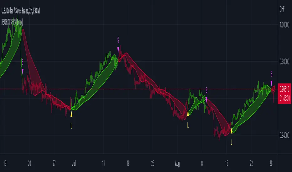
T3 Slope Variation [Loxx]T3 Slope Variation is an indicator that uses T3 moving average to calculate a slope that is then weighted to derive a signal.
The center line
The center line changes color depending on the value of the:
Slope
Signal line
Threshold
If the value is above a signal line (it is not visible on the chart) and the threshold is greater than the required, then the main trend becomes up. And reversed for the trend down.
Colors and style of the histogram
The colors and style of the histogram will be drawn if the value is at the right side, if the above described trend "agrees" with the value (above is green or below zero is red) and if the High is higher than the previous High or Low is lower than the previous low, then the according type of histogram is drawn.
What is the T3 moving average?
Better Moving Averages Tim Tillson
November 1, 1998
Tim Tillson is a software project manager at Hewlett-Packard, with degrees in Mathematics and Computer Science. He has privately traded options and equities for 15 years.
Introduction
"Digital filtering includes the process of smoothing, predicting, differentiating, integrating, separation of signals, and removal of noise from a signal. Thus many people who do such things are actually using digital filters without realizing that they are; being unacquainted with the theory, they neither understand what they have done nor the possibilities of what they might have done."
This quote from R. W. Hamming applies to the vast majority of indicators in technical analysis . Moving averages, be they simple, weighted, or exponential, are lowpass filters; low frequency components in the signal pass through with little attenuation, while high frequencies are severely reduced.
"Oscillator" type indicators (such as MACD , Momentum, Relative Strength Index ) are another type of digital filter called a differentiator.
Tushar Chande has observed that many popular oscillators are highly correlated, which is sensible because they are trying to measure the rate of change of the underlying time series, i.e., are trying to be the first and second derivatives we all learned about in Calculus.
We use moving averages (lowpass filters) in technical analysis to remove the random noise from a time series, to discern the underlying trend or to determine prices at which we will take action. A perfect moving average would have two attributes:
It would be smooth, not sensitive to random noise in the underlying time series. Another way of saying this is that its derivative would not spuriously alternate between positive and negative values.
It would not lag behind the time series it is computed from. Lag, of course, produces late buy or sell signals that kill profits.
The only way one can compute a perfect moving average is to have knowledge of the future, and if we had that, we would buy one lottery ticket a week rather than trade!
Having said this, we can still improve on the conventional simple, weighted, or exponential moving averages. Here's how:
Two Interesting Moving Averages
We will examine two benchmark moving averages based on Linear Regression analysis.
In both cases, a Linear Regression line of length n is fitted to price data.
I call the first moving average ILRS, which stands for Integral of Linear Regression Slope. One simply integrates the slope of a linear regression line as it is successively fitted in a moving window of length n across the data, with the constant of integration being a simple moving average of the first n points. Put another way, the derivative of ILRS is the linear regression slope. Note that ILRS is not the same as a SMA ( simple moving average ) of length n, which is actually the midpoint of the linear regression line as it moves across the data.
We can measure the lag of moving averages with respect to a linear trend by computing how they behave when the input is a line with unit slope. Both SMA (n) and ILRS(n) have lag of n/2, but ILRS is much smoother than SMA .
Our second benchmark moving average is well known, called EPMA or End Point Moving Average. It is the endpoint of the linear regression line of length n as it is fitted across the data. EPMA hugs the data more closely than a simple or exponential moving average of the same length. The price we pay for this is that it is much noisier (less smooth) than ILRS, and it also has the annoying property that it overshoots the data when linear trends are present.
However, EPMA has a lag of 0 with respect to linear input! This makes sense because a linear regression line will fit linear input perfectly, and the endpoint of the LR line will be on the input line.
These two moving averages frame the tradeoffs that we are facing. On one extreme we have ILRS, which is very smooth and has considerable phase lag. EPMA has 0 phase lag, but is too noisy and overshoots. We would like to construct a better moving average which is as smooth as ILRS, but runs closer to where EPMA lies, without the overshoot.
A easy way to attempt this is to split the difference, i.e. use (ILRS(n)+EPMA(n))/2. This will give us a moving average (call it IE /2) which runs in between the two, has phase lag of n/4 but still inherits considerable noise from EPMA. IE /2 is inspirational, however. Can we build something that is comparable, but smoother? Figure 1 shows ILRS, EPMA, and IE /2.
Filter Techniques
Any thoughtful student of filter theory (or resolute experimenter) will have noticed that you can improve the smoothness of a filter by running it through itself multiple times, at the cost of increasing phase lag.
There is a complementary technique (called twicing by J.W. Tukey) which can be used to improve phase lag. If L stands for the operation of running data through a low pass filter, then twicing can be described by:
L' = L(time series) + L(time series - L(time series))
That is, we add a moving average of the difference between the input and the moving average to the moving average. This is algebraically equivalent to:
2L-L(L)
This is the Double Exponential Moving Average or DEMA , popularized by Patrick Mulloy in TASAC (January/February 1994).
In our taxonomy, DEMA has some phase lag (although it exponentially approaches 0) and is somewhat noisy, comparable to IE /2 indicator.
We will use these two techniques to construct our better moving average, after we explore the first one a little more closely.
Fixing Overshoot
An n-day EMA has smoothing constant alpha=2/(n+1) and a lag of (n-1)/2.
Thus EMA (3) has lag 1, and EMA (11) has lag 5. Figure 2 shows that, if I am willing to incur 5 days of lag, I get a smoother moving average if I run EMA (3) through itself 5 times than if I just take EMA (11) once.
This suggests that if EPMA and DEMA have 0 or low lag, why not run fast versions (eg DEMA (3)) through themselves many times to achieve a smooth result? The problem is that multiple runs though these filters increase their tendency to overshoot the data, giving an unusable result. This is because the amplitude response of DEMA and EPMA is greater than 1 at certain frequencies, giving a gain of much greater than 1 at these frequencies when run though themselves multiple times. Figure 3 shows DEMA (7) and EPMA(7) run through themselves 3 times. DEMA^3 has serious overshoot, and EPMA^3 is terrible.
The solution to the overshoot problem is to recall what we are doing with twicing:
DEMA (n) = EMA (n) + EMA (time series - EMA (n))
The second term is adding, in effect, a smooth version of the derivative to the EMA to achieve DEMA . The derivative term determines how hot the moving average's response to linear trends will be. We need to simply turn down the volume to achieve our basic building block:
EMA (n) + EMA (time series - EMA (n))*.7;
This is algebraically the same as:
EMA (n)*1.7-EMA( EMA (n))*.7;
I have chosen .7 as my volume factor, but the general formula (which I call "Generalized Dema") is:
GD (n,v) = EMA (n)*(1+v)-EMA( EMA (n))*v,
Where v ranges between 0 and 1. When v=0, GD is just an EMA , and when v=1, GD is DEMA . In between, GD is a cooler DEMA . By using a value for v less than 1 (I like .7), we cure the multiple DEMA overshoot problem, at the cost of accepting some additional phase delay. Now we can run GD through itself multiple times to define a new, smoother moving average T3 that does not overshoot the data:
T3(n) = GD ( GD ( GD (n)))
In filter theory parlance, T3 is a six-pole non-linear Kalman filter. Kalman filters are ones which use the error (in this case (time series - EMA (n)) to correct themselves. In Technical Analysis , these are called Adaptive Moving Averages; they track the time series more aggressively when it is making large moves.
Included
Alets
Signals
Bar coloring
Loxx's Expanded Source Types
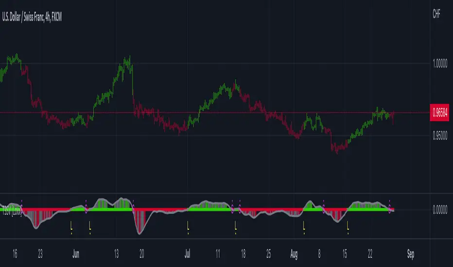
Multi T3 Slopes [Loxx]Multi T3 Slopes is an indicator that checks slopes of 5 (different period) T3 Moving Averages and adds them up to show overall trend. To us this, check for color changes from red to green where there is no red if green is larger than red and there is no red when red is larger than green. When red and green both show up, its a sign of chop.
What is the T3 moving average?
Better Moving Averages Tim Tillson
November 1, 1998
Tim Tillson is a software project manager at Hewlett-Packard, with degrees in Mathematics and Computer Science. He has privately traded options and equities for 15 years.
Introduction
"Digital filtering includes the process of smoothing, predicting, differentiating, integrating, separation of signals, and removal of noise from a signal. Thus many people who do such things are actually using digital filters without realizing that they are; being unacquainted with the theory, they neither understand what they have done nor the possibilities of what they might have done."
This quote from R. W. Hamming applies to the vast majority of indicators in technical analysis . Moving averages, be they simple, weighted, or exponential, are lowpass filters; low frequency components in the signal pass through with little attenuation, while high frequencies are severely reduced.
"Oscillator" type indicators (such as MACD , Momentum, Relative Strength Index ) are another type of digital filter called a differentiator.
Tushar Chande has observed that many popular oscillators are highly correlated, which is sensible because they are trying to measure the rate of change of the underlying time series, i.e., are trying to be the first and second derivatives we all learned about in Calculus.
We use moving averages (lowpass filters) in technical analysis to remove the random noise from a time series, to discern the underlying trend or to determine prices at which we will take action. A perfect moving average would have two attributes:
It would be smooth, not sensitive to random noise in the underlying time series. Another way of saying this is that its derivative would not spuriously alternate between positive and negative values.
It would not lag behind the time series it is computed from. Lag, of course, produces late buy or sell signals that kill profits.
The only way one can compute a perfect moving average is to have knowledge of the future, and if we had that, we would buy one lottery ticket a week rather than trade!
Having said this, we can still improve on the conventional simple, weighted, or exponential moving averages. Here's how:
Two Interesting Moving Averages
We will examine two benchmark moving averages based on Linear Regression analysis.
In both cases, a Linear Regression line of length n is fitted to price data.
I call the first moving average ILRS, which stands for Integral of Linear Regression Slope. One simply integrates the slope of a linear regression line as it is successively fitted in a moving window of length n across the data, with the constant of integration being a simple moving average of the first n points. Put another way, the derivative of ILRS is the linear regression slope. Note that ILRS is not the same as a SMA ( simple moving average ) of length n, which is actually the midpoint of the linear regression line as it moves across the data.
We can measure the lag of moving averages with respect to a linear trend by computing how they behave when the input is a line with unit slope. Both SMA (n) and ILRS(n) have lag of n/2, but ILRS is much smoother than SMA .
Our second benchmark moving average is well known, called EPMA or End Point Moving Average. It is the endpoint of the linear regression line of length n as it is fitted across the data. EPMA hugs the data more closely than a simple or exponential moving average of the same length. The price we pay for this is that it is much noisier (less smooth) than ILRS, and it also has the annoying property that it overshoots the data when linear trends are present.
However, EPMA has a lag of 0 with respect to linear input! This makes sense because a linear regression line will fit linear input perfectly, and the endpoint of the LR line will be on the input line.
These two moving averages frame the tradeoffs that we are facing. On one extreme we have ILRS, which is very smooth and has considerable phase lag. EPMA has 0 phase lag, but is too noisy and overshoots. We would like to construct a better moving average which is as smooth as ILRS, but runs closer to where EPMA lies, without the overshoot.
A easy way to attempt this is to split the difference, i.e. use (ILRS(n)+EPMA(n))/2. This will give us a moving average (call it IE /2) which runs in between the two, has phase lag of n/4 but still inherits considerable noise from EPMA. IE /2 is inspirational, however. Can we build something that is comparable, but smoother? Figure 1 shows ILRS, EPMA, and IE /2.
Filter Techniques
Any thoughtful student of filter theory (or resolute experimenter) will have noticed that you can improve the smoothness of a filter by running it through itself multiple times, at the cost of increasing phase lag.
There is a complementary technique (called twicing by J.W. Tukey) which can be used to improve phase lag. If L stands for the operation of running data through a low pass filter, then twicing can be described by:
L' = L(time series) + L(time series - L(time series))
That is, we add a moving average of the difference between the input and the moving average to the moving average. This is algebraically equivalent to:
2L-L(L)
This is the Double Exponential Moving Average or DEMA , popularized by Patrick Mulloy in TASAC (January/February 1994).
In our taxonomy, DEMA has some phase lag (although it exponentially approaches 0) and is somewhat noisy, comparable to IE /2 indicator.
We will use these two techniques to construct our better moving average, after we explore the first one a little more closely.
Fixing Overshoot
An n-day EMA has smoothing constant alpha=2/(n+1) and a lag of (n-1)/2.
Thus EMA (3) has lag 1, and EMA (11) has lag 5. Figure 2 shows that, if I am willing to incur 5 days of lag, I get a smoother moving average if I run EMA (3) through itself 5 times than if I just take EMA (11) once.
This suggests that if EPMA and DEMA have 0 or low lag, why not run fast versions (eg DEMA (3)) through themselves many times to achieve a smooth result? The problem is that multiple runs though these filters increase their tendency to overshoot the data, giving an unusable result. This is because the amplitude response of DEMA and EPMA is greater than 1 at certain frequencies, giving a gain of much greater than 1 at these frequencies when run though themselves multiple times. Figure 3 shows DEMA (7) and EPMA(7) run through themselves 3 times. DEMA^3 has serious overshoot, and EPMA^3 is terrible.
The solution to the overshoot problem is to recall what we are doing with twicing:
DEMA (n) = EMA (n) + EMA (time series - EMA (n))
The second term is adding, in effect, a smooth version of the derivative to the EMA to achieve DEMA . The derivative term determines how hot the moving average's response to linear trends will be. We need to simply turn down the volume to achieve our basic building block:
EMA (n) + EMA (time series - EMA (n))*.7;
This is algebraically the same as:
EMA (n)*1.7-EMA( EMA (n))*.7;
I have chosen .7 as my volume factor, but the general formula (which I call "Generalized Dema") is:
GD (n,v) = EMA (n)*(1+v)-EMA( EMA (n))*v,
Where v ranges between 0 and 1. When v=0, GD is just an EMA , and when v=1, GD is DEMA . In between, GD is a cooler DEMA . By using a value for v less than 1 (I like .7), we cure the multiple DEMA overshoot problem, at the cost of accepting some additional phase delay. Now we can run GD through itself multiple times to define a new, smoother moving average T3 that does not overshoot the data:
T3(n) = GD ( GD ( GD (n)))
In filter theory parlance, T3 is a six-pole non-linear Kalman filter. Kalman filters are ones which use the error (in this case (time series - EMA (n)) to correct themselves. In Technical Analysis , these are called Adaptive Moving Averages; they track the time series more aggressively when it is making large moves.
Included
Signals: long, short, continuation long, continuation short.
Alerts
Bar coloring
Loxx's expanded source types
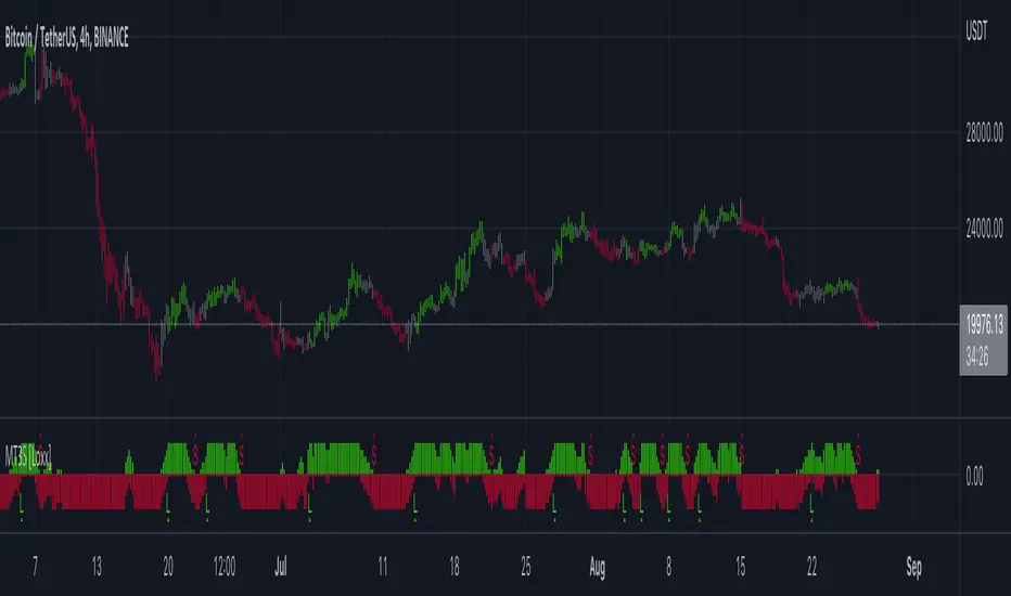
T3 Volatility Quality Index (VQI) w/ DSL & Pips Filtering [Loxx]T3 Volatility Quality Index (VQI) w/ DSL & Pips Filtering is a VQI indicator that uses T3 smoothing and discontinued signal lines to determine breakouts and breakdowns. This also allows filtering by pips.***
What is the Volatility Quality Index ( VQI )?
The idea behind the volatility quality index is to point out the difference between bad and good volatility in order to identify better trade opportunities in the market. This forex indicator works using the True Range algorithm in combination with the open, close, high and low prices.
What are DSL Discontinued Signal Line?
A lot of indicators are using signal lines in order to determine the trend (or some desired state of the indicator) easier. The idea of the signal line is easy : comparing the value to it's smoothed (slightly lagging) state, the idea of current momentum/state is made.
Discontinued signal line is inheriting that simple signal line idea and it is extending it : instead of having one signal line, more lines depending on the current value of the indicator.
"Signal" line is calculated the following way :
When a certain level is crossed into the desired direction, the EMA of that value is calculated for the desired signal line
When that level is crossed into the opposite direction, the previous "signal" line value is simply "inherited" and it becomes a kind of a level
This way it becomes a combination of signal lines and levels that are trying to combine both the good from both methods.
In simple terms, DSL uses the concept of a signal line and betters it by inheriting the previous signal line's value & makes it a level.
What is the T3 moving average?
Better Moving Averages Tim Tillson
November 1, 1998
Tim Tillson is a software project manager at Hewlett-Packard, with degrees in Mathematics and Computer Science. He has privately traded options and equities for 15 years.
Introduction
"Digital filtering includes the process of smoothing, predicting, differentiating, integrating, separation of signals, and removal of noise from a signal. Thus many people who do such things are actually using digital filters without realizing that they are; being unacquainted with the theory, they neither understand what they have done nor the possibilities of what they might have done."
This quote from R. W. Hamming applies to the vast majority of indicators in technical analysis . Moving averages, be they simple, weighted, or exponential, are lowpass filters; low frequency components in the signal pass through with little attenuation, while high frequencies are severely reduced.
"Oscillator" type indicators (such as MACD , Momentum, Relative Strength Index ) are another type of digital filter called a differentiator.
Tushar Chande has observed that many popular oscillators are highly correlated, which is sensible because they are trying to measure the rate of change of the underlying time series, i.e., are trying to be the first and second derivatives we all learned about in Calculus.
We use moving averages (lowpass filters) in technical analysis to remove the random noise from a time series, to discern the underlying trend or to determine prices at which we will take action. A perfect moving average would have two attributes:
It would be smooth, not sensitive to random noise in the underlying time series. Another way of saying this is that its derivative would not spuriously alternate between positive and negative values.
It would not lag behind the time series it is computed from. Lag, of course, produces late buy or sell signals that kill profits.
The only way one can compute a perfect moving average is to have knowledge of the future, and if we had that, we would buy one lottery ticket a week rather than trade!
Having said this, we can still improve on the conventional simple, weighted, or exponential moving averages. Here's how:
Two Interesting Moving Averages
We will examine two benchmark moving averages based on Linear Regression analysis.
In both cases, a Linear Regression line of length n is fitted to price data.
I call the first moving average ILRS, which stands for Integral of Linear Regression Slope. One simply integrates the slope of a linear regression line as it is successively fitted in a moving window of length n across the data, with the constant of integration being a simple moving average of the first n points. Put another way, the derivative of ILRS is the linear regression slope. Note that ILRS is not the same as a SMA ( simple moving average ) of length n, which is actually the midpoint of the linear regression line as it moves across the data.
We can measure the lag of moving averages with respect to a linear trend by computing how they behave when the input is a line with unit slope. Both SMA (n) and ILRS(n) have lag of n/2, but ILRS is much smoother than SMA .
Our second benchmark moving average is well known, called EPMA or End Point Moving Average. It is the endpoint of the linear regression line of length n as it is fitted across the data. EPMA hugs the data more closely than a simple or exponential moving average of the same length. The price we pay for this is that it is much noisier (less smooth) than ILRS, and it also has the annoying property that it overshoots the data when linear trends are present.
However, EPMA has a lag of 0 with respect to linear input! This makes sense because a linear regression line will fit linear input perfectly, and the endpoint of the LR line will be on the input line.
These two moving averages frame the tradeoffs that we are facing. On one extreme we have ILRS, which is very smooth and has considerable phase lag. EPMA has 0 phase lag, but is too noisy and overshoots. We would like to construct a better moving average which is as smooth as ILRS, but runs closer to where EPMA lies, without the overshoot.
A easy way to attempt this is to split the difference, i.e. use (ILRS(n)+EPMA(n))/2. This will give us a moving average (call it IE /2) which runs in between the two, has phase lag of n/4 but still inherits considerable noise from EPMA. IE /2 is inspirational, however. Can we build something that is comparable, but smoother? Figure 1 shows ILRS, EPMA, and IE /2.
Filter Techniques
Any thoughtful student of filter theory (or resolute experimenter) will have noticed that you can improve the smoothness of a filter by running it through itself multiple times, at the cost of increasing phase lag.
There is a complementary technique (called twicing by J.W. Tukey) which can be used to improve phase lag. If L stands for the operation of running data through a low pass filter, then twicing can be described by:
L' = L(time series) + L(time series - L(time series))
That is, we add a moving average of the difference between the input and the moving average to the moving average. This is algebraically equivalent to:
2L-L(L)
This is the Double Exponential Moving Average or DEMA , popularized by Patrick Mulloy in TASAC (January/February 1994).
In our taxonomy, DEMA has some phase lag (although it exponentially approaches 0) and is somewhat noisy, comparable to IE /2 indicator.
We will use these two techniques to construct our better moving average, after we explore the first one a little more closely.
Fixing Overshoot
An n-day EMA has smoothing constant alpha=2/(n+1) and a lag of (n-1)/2.
Thus EMA (3) has lag 1, and EMA (11) has lag 5. Figure 2 shows that, if I am willing to incur 5 days of lag, I get a smoother moving average if I run EMA (3) through itself 5 times than if I just take EMA (11) once.
This suggests that if EPMA and DEMA have 0 or low lag, why not run fast versions (eg DEMA (3)) through themselves many times to achieve a smooth result? The problem is that multiple runs though these filters increase their tendency to overshoot the data, giving an unusable result. This is because the amplitude response of DEMA and EPMA is greater than 1 at certain frequencies, giving a gain of much greater than 1 at these frequencies when run though themselves multiple times. Figure 3 shows DEMA (7) and EPMA(7) run through themselves 3 times. DEMA^3 has serious overshoot, and EPMA^3 is terrible.
The solution to the overshoot problem is to recall what we are doing with twicing:
DEMA (n) = EMA (n) + EMA (time series - EMA (n))
The second term is adding, in effect, a smooth version of the derivative to the EMA to achieve DEMA . The derivative term determines how hot the moving average's response to linear trends will be. We need to simply turn down the volume to achieve our basic building block:
EMA (n) + EMA (time series - EMA (n))*.7;
This is algebraically the same as:
EMA (n)*1.7-EMA( EMA (n))*.7;
I have chosen .7 as my volume factor, but the general formula (which I call "Generalized Dema") is:
GD (n,v) = EMA (n)*(1+v)-EMA( EMA (n))*v,
Where v ranges between 0 and 1. When v=0, GD is just an EMA , and when v=1, GD is DEMA . In between, GD is a cooler DEMA . By using a value for v less than 1 (I like .7), we cure the multiple DEMA overshoot problem, at the cost of accepting some additional phase delay. Now we can run GD through itself multiple times to define a new, smoother moving average T3 that does not overshoot the data:
T3(n) = GD ( GD ( GD (n)))
In filter theory parlance, T3 is a six-pole non-linear Kalman filter. Kalman filters are ones which use the error (in this case (time series - EMA (n)) to correct themselves. In Technical Analysis , these are called Adaptive Moving Averages; they track the time series more aggressively when it is making large moves.
Included
Signals
Alerts
Related indicators
Zero-line Volatility Quality Index (VQI)
Volatility Quality Index w/ Pips Filtering
Variety Moving Average Waddah Attar Explosion (WAE)
***This indicator is tuned to Forex. If you want to make it useful for other tickers, you must change the pip filtering value to match the asset. This means that for BTC, for example, you likely need to use a value of 10,000 or more for pips filter.

VHF-Adaptive T3 iTrend [Loxx]VHF-Adaptive T3 iTrend is an iTrend indicator with T3 smoothing and Vertical Horizontal Filter Adaptive period input. iTrend is used to determine where the trend starts and ends. You'll notice that the noise filter on this one is extreme. Adjust the period inputs accordingly to suit your take and your backtest requirements. This is also useful for scalping lower timeframes. Enjoy!
What is VHF Adaptive Period?
Vertical Horizontal Filter (VHF) was created by Adam White to identify trending and ranging markets. VHF measures the level of trend activity, similar to ADX DI. Vertical Horizontal Filter does not, itself, generate trading signals, but determines whether signals are taken from trend or momentum indicators. Using this trend information, one is then able to derive an average cycle length.
What is the T3 moving average?
Better Moving Averages Tim Tillson
November 1, 1998
Tim Tillson is a software project manager at Hewlett-Packard, with degrees in Mathematics and Computer Science. He has privately traded options and equities for 15 years.
Introduction
"Digital filtering includes the process of smoothing, predicting, differentiating, integrating, separation of signals, and removal of noise from a signal. Thus many people who do such things are actually using digital filters without realizing that they are; being unacquainted with the theory, they neither understand what they have done nor the possibilities of what they might have done."
This quote from R. W. Hamming applies to the vast majority of indicators in technical analysis . Moving averages, be they simple, weighted, or exponential, are lowpass filters; low frequency components in the signal pass through with little attenuation, while high frequencies are severely reduced.
"Oscillator" type indicators (such as MACD , Momentum, Relative Strength Index ) are another type of digital filter called a differentiator.
Tushar Chande has observed that many popular oscillators are highly correlated, which is sensible because they are trying to measure the rate of change of the underlying time series, i.e., are trying to be the first and second derivatives we all learned about in Calculus.
We use moving averages (lowpass filters) in technical analysis to remove the random noise from a time series, to discern the underlying trend or to determine prices at which we will take action. A perfect moving average would have two attributes:
It would be smooth, not sensitive to random noise in the underlying time series. Another way of saying this is that its derivative would not spuriously alternate between positive and negative values.
It would not lag behind the time series it is computed from. Lag, of course, produces late buy or sell signals that kill profits.
The only way one can compute a perfect moving average is to have knowledge of the future, and if we had that, we would buy one lottery ticket a week rather than trade!
Having said this, we can still improve on the conventional simple, weighted, or exponential moving averages. Here's how:
Two Interesting Moving Averages
We will examine two benchmark moving averages based on Linear Regression analysis.
In both cases, a Linear Regression line of length n is fitted to price data.
I call the first moving average ILRS, which stands for Integral of Linear Regression Slope. One simply integrates the slope of a linear regression line as it is successively fitted in a moving window of length n across the data, with the constant of integration being a simple moving average of the first n points. Put another way, the derivative of ILRS is the linear regression slope. Note that ILRS is not the same as a SMA ( simple moving average ) of length n, which is actually the midpoint of the linear regression line as it moves across the data.
We can measure the lag of moving averages with respect to a linear trend by computing how they behave when the input is a line with unit slope. Both SMA (n) and ILRS(n) have lag of n/2, but ILRS is much smoother than SMA .
Our second benchmark moving average is well known, called EPMA or End Point Moving Average. It is the endpoint of the linear regression line of length n as it is fitted across the data. EPMA hugs the data more closely than a simple or exponential moving average of the same length. The price we pay for this is that it is much noisier (less smooth) than ILRS, and it also has the annoying property that it overshoots the data when linear trends are present.
However, EPMA has a lag of 0 with respect to linear input! This makes sense because a linear regression line will fit linear input perfectly, and the endpoint of the LR line will be on the input line.
These two moving averages frame the tradeoffs that we are facing. On one extreme we have ILRS, which is very smooth and has considerable phase lag. EPMA has 0 phase lag, but is too noisy and overshoots. We would like to construct a better moving average which is as smooth as ILRS, but runs closer to where EPMA lies, without the overshoot.
A easy way to attempt this is to split the difference, i.e. use (ILRS(n)+EPMA(n))/2. This will give us a moving average (call it IE /2) which runs in between the two, has phase lag of n/4 but still inherits considerable noise from EPMA. IE /2 is inspirational, however. Can we build something that is comparable, but smoother? Figure 1 shows ILRS, EPMA, and IE /2.
Filter Techniques
Any thoughtful student of filter theory (or resolute experimenter) will have noticed that you can improve the smoothness of a filter by running it through itself multiple times, at the cost of increasing phase lag.
There is a complementary technique (called twicing by J.W. Tukey) which can be used to improve phase lag. If L stands for the operation of running data through a low pass filter, then twicing can be described by:
L' = L(time series) + L(time series - L(time series))
That is, we add a moving average of the difference between the input and the moving average to the moving average. This is algebraically equivalent to:
2L-L(L)
This is the Double Exponential Moving Average or DEMA , popularized by Patrick Mulloy in TASAC (January/February 1994).
In our taxonomy, DEMA has some phase lag (although it exponentially approaches 0) and is somewhat noisy, comparable to IE /2 indicator.
We will use these two techniques to construct our better moving average, after we explore the first one a little more closely.
Fixing Overshoot
An n-day EMA has smoothing constant alpha=2/(n+1) and a lag of (n-1)/2.
Thus EMA (3) has lag 1, and EMA (11) has lag 5. Figure 2 shows that, if I am willing to incur 5 days of lag, I get a smoother moving average if I run EMA (3) through itself 5 times than if I just take EMA (11) once.
This suggests that if EPMA and DEMA have 0 or low lag, why not run fast versions (eg DEMA (3)) through themselves many times to achieve a smooth result? The problem is that multiple runs though these filters increase their tendency to overshoot the data, giving an unusable result. This is because the amplitude response of DEMA and EPMA is greater than 1 at certain frequencies, giving a gain of much greater than 1 at these frequencies when run though themselves multiple times. Figure 3 shows DEMA (7) and EPMA(7) run through themselves 3 times. DEMA^3 has serious overshoot, and EPMA^3 is terrible.
The solution to the overshoot problem is to recall what we are doing with twicing:
DEMA (n) = EMA (n) + EMA (time series - EMA (n))
The second term is adding, in effect, a smooth version of the derivative to the EMA to achieve DEMA . The derivative term determines how hot the moving average's response to linear trends will be. We need to simply turn down the volume to achieve our basic building block:
EMA (n) + EMA (time series - EMA (n))*.7;
This is algebraically the same as:
EMA (n)*1.7-EMA( EMA (n))*.7;
I have chosen .7 as my volume factor, but the general formula (which I call "Generalized Dema") is:
GD (n,v) = EMA (n)*(1+v)-EMA( EMA (n))*v,
Where v ranges between 0 and 1. When v=0, GD is just an EMA , and when v=1, GD is DEMA . In between, GD is a cooler DEMA . By using a value for v less than 1 (I like .7), we cure the multiple DEMA overshoot problem, at the cost of accepting some additional phase delay. Now we can run GD through itself multiple times to define a new, smoother moving average T3 that does not overshoot the data:
T3(n) = GD ( GD ( GD (n)))
In filter theory parlance, T3 is a six-pole non-linear Kalman filter. Kalman filters are ones which use the error (in this case (time series - EMA (n)) to correct themselves. In Technical Analysis , these are called Adaptive Moving Averages; they track the time series more aggressively when it is making large moves.
Included
Bar coloring
Alerts
Signals
Loxx's Expanded Source Types
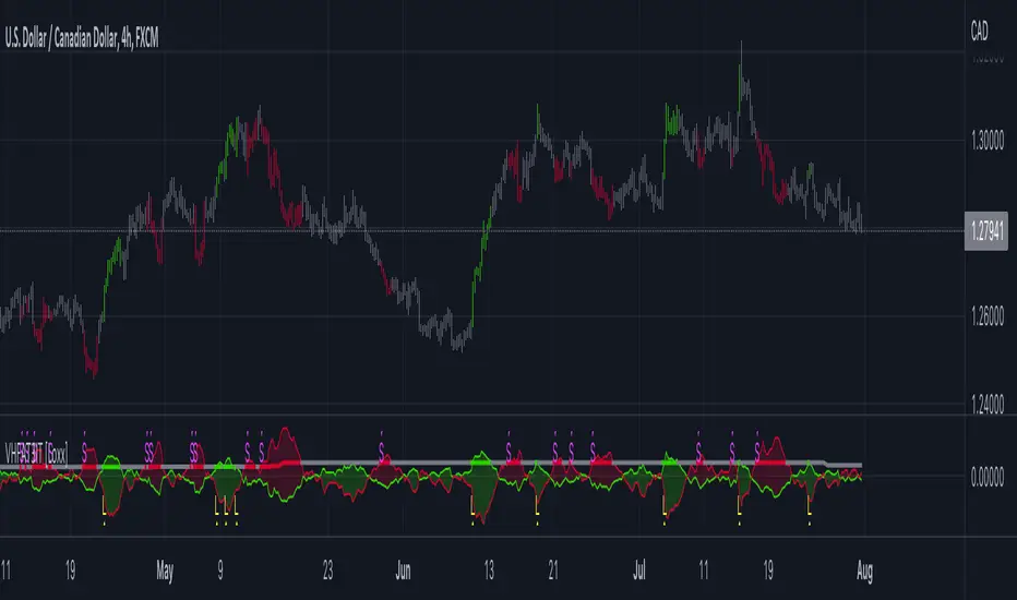
CFB-Adaptive CCI w/ T3 Smoothing [Loxx]CFB-Adaptive CCI w/ T3 Smoothing is a CCI indicator with adaptive period inputs and T3 smoothing. Jurik's Composite Fractal Behavior is used to created dynamic period input.
What is Composite Fractal Behavior ( CFB )?
All around you mechanisms adjust themselves to their environment. From simple thermostats that react to air temperature to computer chips in modern cars that respond to changes in engine temperature, r.p.m.'s, torque, and throttle position. It was only a matter of time before fast desktop computers applied the mathematics of self-adjustment to systems that trade the financial markets.
Unlike basic systems with fixed formulas, an adaptive system adjusts its own equations. For example, start with a basic channel breakout system that uses the highest closing price of the last N bars as a threshold for detecting breakouts on the up side. An adaptive and improved version of this system would adjust N according to market conditions, such as momentum, price volatility or acceleration.
Since many systems are based directly or indirectly on cycles, another useful measure of market condition is the periodic length of a price chart's dominant cycle, (DC), that cycle with the greatest influence on price action.
The utility of this new DC measure was noted by author Murray Ruggiero in the January '96 issue of Futures Magazine. In it. Mr. Ruggiero used it to adaptive adjust the value of N in a channel breakout system. He then simulated trading 15 years of D-Mark futures in order to compare its performance to a similar system that had a fixed optimal value of N. The adaptive version produced 20% more profit!
This DC index utilized the popular MESA algorithm (a formulation by John Ehlers adapted from Burg's maximum entropy algorithm, MEM). Unfortunately, the DC approach is problematic when the market has no real dominant cycle momentum, because the mathematics will produce a value whether or not one actually exists! Therefore, we developed a proprietary indicator that does not presuppose the presence of market cycles. It's called CFB (Composite Fractal Behavior) and it works well whether or not the market is cyclic.
CFB examines price action for a particular fractal pattern, categorizes them by size, and then outputs a composite fractal size index. This index is smooth, timely and accurate
Essentially, CFB reveals the length of the market's trending action time frame. Long trending activity produces a large CFB index and short choppy action produces a small index value. Investors have found many applications for CFB which involve scaling other existing technical indicators adaptively, on a bar-to-bar basis.
What is Jurik Volty used in the Juirk Filter?
One of the lesser known qualities of Juirk smoothing is that the Jurik smoothing process is adaptive. "Jurik Volty" (a sort of market volatility ) is what makes Jurik smoothing adaptive. The Jurik Volty calculation can be used as both a standalone indicator and to smooth other indicators that you wish to make adaptive.
What is the Jurik Moving Average?
Have you noticed how moving averages add some lag (delay) to your signals? ... especially when price gaps up or down in a big move, and you are waiting for your moving average to catch up? Wait no more! JMA eliminates this problem forever and gives you the best of both worlds: low lag and smooth lines.
Ideally, you would like a filtered signal to be both smooth and lag-free. Lag causes delays in your trades, and increasing lag in your indicators typically result in lower profits. In other words, late comers get what's left on the table after the feast has already begun.
What is the T3 moving average?
Better Moving Averages Tim Tillson
November 1, 1998
Tim Tillson is a software project manager at Hewlett-Packard, with degrees in Mathematics and Computer Science. He has privately traded options and equities for 15 years.
Introduction
"Digital filtering includes the process of smoothing, predicting, differentiating, integrating, separation of signals, and removal of noise from a signal. Thus many people who do such things are actually using digital filters without realizing that they are; being unacquainted with the theory, they neither understand what they have done nor the possibilities of what they might have done."
This quote from R. W. Hamming applies to the vast majority of indicators in technical analysis . Moving averages, be they simple, weighted, or exponential, are lowpass filters; low frequency components in the signal pass through with little attenuation, while high frequencies are severely reduced.
"Oscillator" type indicators (such as MACD , Momentum, Relative Strength Index ) are another type of digital filter called a differentiator.
Tushar Chande has observed that many popular oscillators are highly correlated, which is sensible because they are trying to measure the rate of change of the underlying time series, i.e., are trying to be the first and second derivatives we all learned about in Calculus.
We use moving averages (lowpass filters) in technical analysis to remove the random noise from a time series, to discern the underlying trend or to determine prices at which we will take action. A perfect moving average would have two attributes:
It would be smooth, not sensitive to random noise in the underlying time series. Another way of saying this is that its derivative would not spuriously alternate between positive and negative values.
It would not lag behind the time series it is computed from. Lag, of course, produces late buy or sell signals that kill profits.
The only way one can compute a perfect moving average is to have knowledge of the future, and if we had that, we would buy one lottery ticket a week rather than trade!
Having said this, we can still improve on the conventional simple, weighted, or exponential moving averages. Here's how:
Two Interesting Moving Averages
We will examine two benchmark moving averages based on Linear Regression analysis.
In both cases, a Linear Regression line of length n is fitted to price data.
I call the first moving average ILRS, which stands for Integral of Linear Regression Slope. One simply integrates the slope of a linear regression line as it is successively fitted in a moving window of length n across the data, with the constant of integration being a simple moving average of the first n points. Put another way, the derivative of ILRS is the linear regression slope. Note that ILRS is not the same as a SMA ( simple moving average ) of length n, which is actually the midpoint of the linear regression line as it moves across the data.
We can measure the lag of moving averages with respect to a linear trend by computing how they behave when the input is a line with unit slope. Both SMA (n) and ILRS(n) have lag of n/2, but ILRS is much smoother than SMA .
Our second benchmark moving average is well known, called EPMA or End Point Moving Average. It is the endpoint of the linear regression line of length n as it is fitted across the data. EPMA hugs the data more closely than a simple or exponential moving average of the same length. The price we pay for this is that it is much noisier (less smooth) than ILRS, and it also has the annoying property that it overshoots the data when linear trends are present.
However, EPMA has a lag of 0 with respect to linear input! This makes sense because a linear regression line will fit linear input perfectly, and the endpoint of the LR line will be on the input line.
These two moving averages frame the tradeoffs that we are facing. On one extreme we have ILRS, which is very smooth and has considerable phase lag. EPMA has 0 phase lag, but is too noisy and overshoots. We would like to construct a better moving average which is as smooth as ILRS, but runs closer to where EPMA lies, without the overshoot.
A easy way to attempt this is to split the difference, i.e. use (ILRS(n)+EPMA(n))/2. This will give us a moving average (call it IE /2) which runs in between the two, has phase lag of n/4 but still inherits considerable noise from EPMA. IE /2 is inspirational, however. Can we build something that is comparable, but smoother? Figure 1 shows ILRS, EPMA, and IE /2.
Filter Techniques
Any thoughtful student of filter theory (or resolute experimenter) will have noticed that you can improve the smoothness of a filter by running it through itself multiple times, at the cost of increasing phase lag.
There is a complementary technique (called twicing by J.W. Tukey) which can be used to improve phase lag. If L stands for the operation of running data through a low pass filter, then twicing can be described by:
L' = L(time series) + L(time series - L(time series))
That is, we add a moving average of the difference between the input and the moving average to the moving average. This is algebraically equivalent to:
2L-L(L)
This is the Double Exponential Moving Average or DEMA , popularized by Patrick Mulloy in TASAC (January/February 1994).
In our taxonomy, DEMA has some phase lag (although it exponentially approaches 0) and is somewhat noisy, comparable to IE /2 indicator.
We will use these two techniques to construct our better moving average, after we explore the first one a little more closely.
Fixing Overshoot
An n-day EMA has smoothing constant alpha=2/(n+1) and a lag of (n-1)/2.
Thus EMA (3) has lag 1, and EMA (11) has lag 5. Figure 2 shows that, if I am willing to incur 5 days of lag, I get a smoother moving average if I run EMA (3) through itself 5 times than if I just take EMA (11) once.
This suggests that if EPMA and DEMA have 0 or low lag, why not run fast versions (eg DEMA (3)) through themselves many times to achieve a smooth result? The problem is that multiple runs though these filters increase their tendency to overshoot the data, giving an unusable result. This is because the amplitude response of DEMA and EPMA is greater than 1 at certain frequencies, giving a gain of much greater than 1 at these frequencies when run though themselves multiple times. Figure 3 shows DEMA (7) and EPMA(7) run through themselves 3 times. DEMA^3 has serious overshoot, and EPMA^3 is terrible.
The solution to the overshoot problem is to recall what we are doing with twicing:
DEMA (n) = EMA (n) + EMA (time series - EMA (n))
The second term is adding, in effect, a smooth version of the derivative to the EMA to achieve DEMA . The derivative term determines how hot the moving average's response to linear trends will be. We need to simply turn down the volume to achieve our basic building block:
EMA (n) + EMA (time series - EMA (n))*.7;
This is algebraically the same as:
EMA (n)*1.7-EMA( EMA (n))*.7;
I have chosen .7 as my volume factor, but the general formula (which I call "Generalized Dema") is:
GD (n,v) = EMA (n)*(1+v)-EMA( EMA (n))*v,
Where v ranges between 0 and 1. When v=0, GD is just an EMA , and when v=1, GD is DEMA . In between, GD is a cooler DEMA . By using a value for v less than 1 (I like .7), we cure the multiple DEMA overshoot problem, at the cost of accepting some additional phase delay. Now we can run GD through itself multiple times to define a new, smoother moving average T3 that does not overshoot the data:
T3(n) = GD ( GD ( GD (n)))
In filter theory parlance, T3 is a six-pole non-linear Kalman filter. Kalman filters are ones which use the error (in this case (time series - EMA (n)) to correct themselves. In Technical Analysis , these are called Adaptive Moving Averages; they track the time series more aggressively when it is making large moves.
Included:
Bar coloring
Signals
Alerts

STD-Adaptive T3 Channel w/ Ehlers Swiss Army Knife Mod. [Loxx]STD-Adaptive T3 Channel w/ Ehlers Swiss Army Knife Mod. is an adaptive T3 indicator using standard deviation adaptivity and Ehlers Swiss Army Knife indicator to adjust the alpha value of the T3 calculation. This helps identify trends and reduce noise. In addition. I've included a Keltner Channel to show reversal/exhaustion zones.
What is the Swiss Army Knife Indicator?
John Ehlers explains the calculation here: www.mesasoftware.com
What is the T3 moving average?
Better Moving Averages Tim Tillson
November 1, 1998
Tim Tillson is a software project manager at Hewlett-Packard, with degrees in Mathematics and Computer Science. He has privately traded options and equities for 15 years.
Introduction
"Digital filtering includes the process of smoothing, predicting, differentiating, integrating, separation of signals, and removal of noise from a signal. Thus many people who do such things are actually using digital filters without realizing that they are; being unacquainted with the theory, they neither understand what they have done nor the possibilities of what they might have done."
This quote from R. W. Hamming applies to the vast majority of indicators in technical analysis . Moving averages, be they simple, weighted, or exponential, are lowpass filters; low frequency components in the signal pass through with little attenuation, while high frequencies are severely reduced.
"Oscillator" type indicators (such as MACD , Momentum, Relative Strength Index ) are another type of digital filter called a differentiator.
Tushar Chande has observed that many popular oscillators are highly correlated, which is sensible because they are trying to measure the rate of change of the underlying time series, i.e., are trying to be the first and second derivatives we all learned about in Calculus.
We use moving averages (lowpass filters) in technical analysis to remove the random noise from a time series, to discern the underlying trend or to determine prices at which we will take action. A perfect moving average would have two attributes:
It would be smooth, not sensitive to random noise in the underlying time series. Another way of saying this is that its derivative would not spuriously alternate between positive and negative values.
It would not lag behind the time series it is computed from. Lag, of course, produces late buy or sell signals that kill profits.
The only way one can compute a perfect moving average is to have knowledge of the future, and if we had that, we would buy one lottery ticket a week rather than trade!
Having said this, we can still improve on the conventional simple, weighted, or exponential moving averages. Here's how:
Two Interesting Moving Averages
We will examine two benchmark moving averages based on Linear Regression analysis.
In both cases, a Linear Regression line of length n is fitted to price data.
I call the first moving average ILRS, which stands for Integral of Linear Regression Slope. One simply integrates the slope of a linear regression line as it is successively fitted in a moving window of length n across the data, with the constant of integration being a simple moving average of the first n points. Put another way, the derivative of ILRS is the linear regression slope. Note that ILRS is not the same as a SMA ( simple moving average ) of length n, which is actually the midpoint of the linear regression line as it moves across the data.
We can measure the lag of moving averages with respect to a linear trend by computing how they behave when the input is a line with unit slope. Both SMA (n) and ILRS(n) have lag of n/2, but ILRS is much smoother than SMA .
Our second benchmark moving average is well known, called EPMA or End Point Moving Average. It is the endpoint of the linear regression line of length n as it is fitted across the data. EPMA hugs the data more closely than a simple or exponential moving average of the same length. The price we pay for this is that it is much noisier (less smooth) than ILRS, and it also has the annoying property that it overshoots the data when linear trends are present.
However, EPMA has a lag of 0 with respect to linear input! This makes sense because a linear regression line will fit linear input perfectly, and the endpoint of the LR line will be on the input line.
These two moving averages frame the tradeoffs that we are facing. On one extreme we have ILRS, which is very smooth and has considerable phase lag. EPMA has 0 phase lag, but is too noisy and overshoots. We would like to construct a better moving average which is as smooth as ILRS, but runs closer to where EPMA lies, without the overshoot.
A easy way to attempt this is to split the difference, i.e. use (ILRS(n)+EPMA(n))/2. This will give us a moving average (call it IE /2) which runs in between the two, has phase lag of n/4 but still inherits considerable noise from EPMA. IE /2 is inspirational, however. Can we build something that is comparable, but smoother? Figure 1 shows ILRS, EPMA, and IE /2.
Filter Techniques
Any thoughtful student of filter theory (or resolute experimenter) will have noticed that you can improve the smoothness of a filter by running it through itself multiple times, at the cost of increasing phase lag.
There is a complementary technique (called twicing by J.W. Tukey) which can be used to improve phase lag. If L stands for the operation of running data through a low pass filter, then twicing can be described by:
L' = L(time series) + L(time series - L(time series))
That is, we add a moving average of the difference between the input and the moving average to the moving average. This is algebraically equivalent to:
2L-L(L)
This is the Double Exponential Moving Average or DEMA , popularized by Patrick Mulloy in TASAC (January/February 1994).
In our taxonomy, DEMA has some phase lag (although it exponentially approaches 0) and is somewhat noisy, comparable to IE /2 indicator.
We will use these two techniques to construct our better moving average, after we explore the first one a little more closely.
Fixing Overshoot
An n-day EMA has smoothing constant alpha=2/(n+1) and a lag of (n-1)/2.
Thus EMA (3) has lag 1, and EMA (11) has lag 5. Figure 2 shows that, if I am willing to incur 5 days of lag, I get a smoother moving average if I run EMA (3) through itself 5 times than if I just take EMA (11) once.
This suggests that if EPMA and DEMA have 0 or low lag, why not run fast versions (eg DEMA (3)) through themselves many times to achieve a smooth result? The problem is that multiple runs though these filters increase their tendency to overshoot the data, giving an unusable result. This is because the amplitude response of DEMA and EPMA is greater than 1 at certain frequencies, giving a gain of much greater than 1 at these frequencies when run though themselves multiple times. Figure 3 shows DEMA (7) and EPMA(7) run through themselves 3 times. DEMA^3 has serious overshoot, and EPMA^3 is terrible.
The solution to the overshoot problem is to recall what we are doing with twicing:
DEMA (n) = EMA (n) + EMA (time series - EMA (n))
The second term is adding, in effect, a smooth version of the derivative to the EMA to achieve DEMA . The derivative term determines how hot the moving average's response to linear trends will be. We need to simply turn down the volume to achieve our basic building block:
EMA (n) + EMA (time series - EMA (n))*.7;
This is algebraically the same as:
EMA (n)*1.7-EMA( EMA (n))*.7;
I have chosen .7 as my volume factor, but the general formula (which I call "Generalized Dema") is:
GD (n,v) = EMA (n)*(1+v)-EMA( EMA (n))*v,
Where v ranges between 0 and 1. When v=0, GD is just an EMA , and when v=1, GD is DEMA . In between, GD is a cooler DEMA . By using a value for v less than 1 (I like .7), we cure the multiple DEMA overshoot problem, at the cost of accepting some additional phase delay. Now we can run GD through itself multiple times to define a new, smoother moving average T3 that does not overshoot the data:
T3(n) = GD ( GD ( GD (n)))
In filter theory parlance, T3 is a six-pole non-linear Kalman filter. Kalman filters are ones which use the error (in this case (time series - EMA (n)) to correct themselves. In Technical Analysis , these are called Adaptive Moving Averages; they track the time series more aggressively when it is making large moves.
Included:
Bar coloring
Signals
Alerts
Loxx's Expanded Source Types
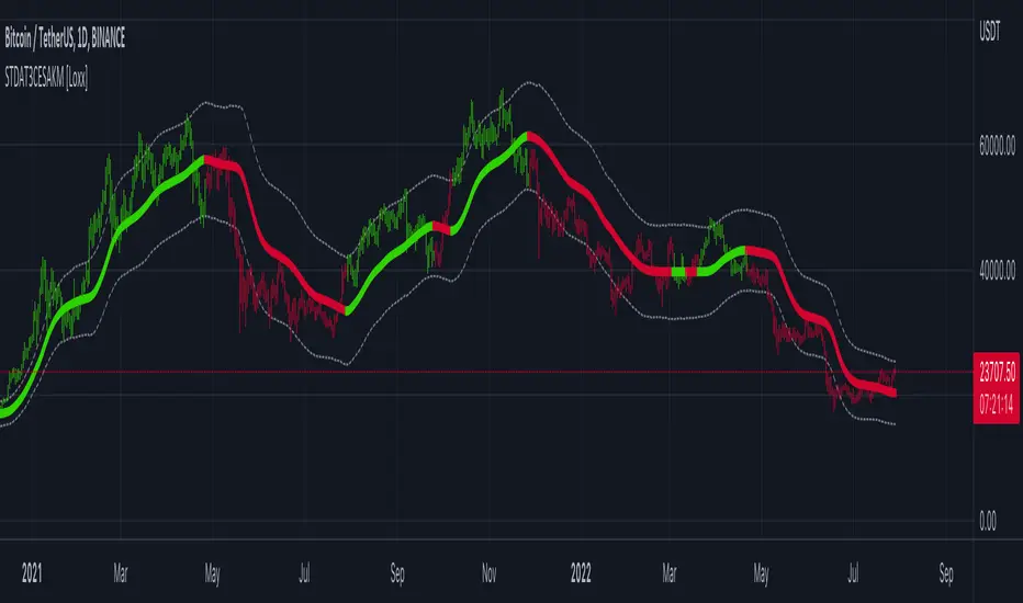
T3 Velocity [Loxx]T3 Velocity is a simple velocity indicator using T3 moving average that uses gradient colors to better identify trends.
What is the T3 moving average?
Better Moving Averages Tim Tillson
November 1, 1998
Tim Tillson is a software project manager at Hewlett-Packard, with degrees in Mathematics and Computer Science. He has privately traded options and equities for 15 years.
Introduction
"Digital filtering includes the process of smoothing, predicting, differentiating, integrating, separation of signals, and removal of noise from a signal. Thus many people who do such things are actually using digital filters without realizing that they are; being unacquainted with the theory, they neither understand what they have done nor the possibilities of what they might have done."
This quote from R. W. Hamming applies to the vast majority of indicators in technical analysis . Moving averages, be they simple, weighted, or exponential, are lowpass filters; low frequency components in the signal pass through with little attenuation, while high frequencies are severely reduced.
"Oscillator" type indicators (such as MACD , Momentum, Relative Strength Index ) are another type of digital filter called a differentiator.
Tushar Chande has observed that many popular oscillators are highly correlated, which is sensible because they are trying to measure the rate of change of the underlying time series, i.e., are trying to be the first and second derivatives we all learned about in Calculus.
We use moving averages (lowpass filters) in technical analysis to remove the random noise from a time series, to discern the underlying trend or to determine prices at which we will take action. A perfect moving average would have two attributes:
It would be smooth, not sensitive to random noise in the underlying time series. Another way of saying this is that its derivative would not spuriously alternate between positive and negative values.
It would not lag behind the time series it is computed from. Lag, of course, produces late buy or sell signals that kill profits.
The only way one can compute a perfect moving average is to have knowledge of the future, and if we had that, we would buy one lottery ticket a week rather than trade!
Having said this, we can still improve on the conventional simple, weighted, or exponential moving averages. Here's how:
Two Interesting Moving Averages
We will examine two benchmark moving averages based on Linear Regression analysis.
In both cases, a Linear Regression line of length n is fitted to price data.
I call the first moving average ILRS, which stands for Integral of Linear Regression Slope. One simply integrates the slope of a linear regression line as it is successively fitted in a moving window of length n across the data, with the constant of integration being a simple moving average of the first n points. Put another way, the derivative of ILRS is the linear regression slope. Note that ILRS is not the same as a SMA ( simple moving average ) of length n, which is actually the midpoint of the linear regression line as it moves across the data.
We can measure the lag of moving averages with respect to a linear trend by computing how they behave when the input is a line with unit slope. Both SMA (n) and ILRS(n) have lag of n/2, but ILRS is much smoother than SMA .
Our second benchmark moving average is well known, called EPMA or End Point Moving Average. It is the endpoint of the linear regression line of length n as it is fitted across the data. EPMA hugs the data more closely than a simple or exponential moving average of the same length. The price we pay for this is that it is much noisier (less smooth) than ILRS, and it also has the annoying property that it overshoots the data when linear trends are present.
However, EPMA has a lag of 0 with respect to linear input! This makes sense because a linear regression line will fit linear input perfectly, and the endpoint of the LR line will be on the input line.
These two moving averages frame the tradeoffs that we are facing. On one extreme we have ILRS, which is very smooth and has considerable phase lag. EPMA has 0 phase lag, but is too noisy and overshoots. We would like to construct a better moving average which is as smooth as ILRS, but runs closer to where EPMA lies, without the overshoot.
A easy way to attempt this is to split the difference, i.e. use (ILRS(n)+EPMA(n))/2. This will give us a moving average (call it IE /2) which runs in between the two, has phase lag of n/4 but still inherits considerable noise from EPMA. IE /2 is inspirational, however. Can we build something that is comparable, but smoother? Figure 1 shows ILRS, EPMA, and IE /2.
Filter Techniques
Any thoughtful student of filter theory (or resolute experimenter) will have noticed that you can improve the smoothness of a filter by running it through itself multiple times, at the cost of increasing phase lag.
There is a complementary technique (called twicing by J.W. Tukey) which can be used to improve phase lag. If L stands for the operation of running data through a low pass filter, then twicing can be described by:
L' = L(time series) + L(time series - L(time series))
That is, we add a moving average of the difference between the input and the moving average to the moving average. This is algebraically equivalent to:
2L-L(L)
This is the Double Exponential Moving Average or DEMA , popularized by Patrick Mulloy in TASAC (January/February 1994).
In our taxonomy, DEMA has some phase lag (although it exponentially approaches 0) and is somewhat noisy, comparable to IE /2 indicator.
We will use these two techniques to construct our better moving average, after we explore the first one a little more closely.
Fixing Overshoot
An n-day EMA has smoothing constant alpha=2/(n+1) and a lag of (n-1)/2.
Thus EMA (3) has lag 1, and EMA (11) has lag 5. Figure 2 shows that, if I am willing to incur 5 days of lag, I get a smoother moving average if I run EMA (3) through itself 5 times than if I just take EMA (11) once.
This suggests that if EPMA and DEMA have 0 or low lag, why not run fast versions (eg DEMA (3)) through themselves many times to achieve a smooth result? The problem is that multiple runs though these filters increase their tendency to overshoot the data, giving an unusable result. This is because the amplitude response of DEMA and EPMA is greater than 1 at certain frequencies, giving a gain of much greater than 1 at these frequencies when run though themselves multiple times. Figure 3 shows DEMA (7) and EPMA(7) run through themselves 3 times. DEMA^3 has serious overshoot, and EPMA^3 is terrible.
The solution to the overshoot problem is to recall what we are doing with twicing:
DEMA (n) = EMA (n) + EMA (time series - EMA (n))
The second term is adding, in effect, a smooth version of the derivative to the EMA to achieve DEMA . The derivative term determines how hot the moving average's response to linear trends will be. We need to simply turn down the volume to achieve our basic building block:
EMA (n) + EMA (time series - EMA (n))*.7;
This is algebraically the same as:
EMA (n)*1.7-EMA( EMA (n))*.7;
I have chosen .7 as my volume factor, but the general formula (which I call "Generalized Dema") is:
GD (n,v) = EMA (n)*(1+v)-EMA( EMA (n))*v,
Where v ranges between 0 and 1. When v=0, GD is just an EMA , and when v=1, GD is DEMA . In between, GD is a cooler DEMA . By using a value for v less than 1 (I like .7), we cure the multiple DEMA overshoot problem, at the cost of accepting some additional phase delay. Now we can run GD through itself multiple times to define a new, smoother moving average T3 that does not overshoot the data:
T3(n) = GD ( GD ( GD (n)))
In filter theory parlance, T3 is a six-pole non-linear Kalman filter. Kalman filters are ones which use the error (in this case (time series - EMA (n)) to correct themselves. In Technical Analysis , these are called Adaptive Moving Averages; they track the time series more aggressively when it is making large moves.
Included:
Bar coloring
Signals
Alerts
Loxx's Expanded Source Types

R-squared Adaptive T3 w/ DSL [Loxx]R-squared Adaptive T3 w/ DSL is the following T3 indicator but with Discontinued Signal Lines added to reduce noise and thereby increase signal accuracy. This adaptation makes this indicator lower TF scalp friendly.
What is R-squared Adaptive?
One tool available in forecasting the trendiness of the breakout is the coefficient of determination ( R-squared ), a statistical measurement.
The R-squared indicates linear strength between the security's price (the Y - axis) and time (the X - axis). The R-squared is the percentage of squared error that the linear regression can eliminate if it were used as the predictor instead of the mean value. If the R-squared were 0.99, then the linear regression would eliminate 99% of the error for prediction versus predicting closing prices using a simple moving average .
R-squared is used here to derive a T3 factor used to modify price before passing price through a six-pole non-linear Kalman filter.
What is the T3 moving average?
Better Moving Averages Tim Tillson
November 1, 1998
Tim Tillson is a software project manager at Hewlett-Packard, with degrees in Mathematics and Computer Science. He has privately traded options and equities for 15 years.
Introduction
"Digital filtering includes the process of smoothing, predicting, differentiating, integrating, separation of signals, and removal of noise from a signal. Thus many people who do such things are actually using digital filters without realizing that they are; being unacquainted with the theory, they neither understand what they have done nor the possibilities of what they might have done."
This quote from R. W. Hamming applies to the vast majority of indicators in technical analysis . Moving averages, be they simple, weighted, or exponential, are lowpass filters; low frequency components in the signal pass through with little attenuation, while high frequencies are severely reduced.
"Oscillator" type indicators (such as MACD , Momentum, Relative Strength Index ) are another type of digital filter called a differentiator.
Tushar Chande has observed that many popular oscillators are highly correlated, which is sensible because they are trying to measure the rate of change of the underlying time series, i.e., are trying to be the first and second derivatives we all learned about in Calculus.
We use moving averages (lowpass filters) in technical analysis to remove the random noise from a time series, to discern the underlying trend or to determine prices at which we will take action. A perfect moving average would have two attributes:
It would be smooth, not sensitive to random noise in the underlying time series. Another way of saying this is that its derivative would not spuriously alternate between positive and negative values.
It would not lag behind the time series it is computed from. Lag, of course, produces late buy or sell signals that kill profits.
The only way one can compute a perfect moving average is to have knowledge of the future, and if we had that, we would buy one lottery ticket a week rather than trade!
Having said this, we can still improve on the conventional simple, weighted, or exponential moving averages. Here's how:
Two Interesting Moving Averages
We will examine two benchmark moving averages based on Linear Regression analysis.
In both cases, a Linear Regression line of length n is fitted to price data.
I call the first moving average ILRS, which stands for Integral of Linear Regression Slope. One simply integrates the slope of a linear regression line as it is successively fitted in a moving window of length n across the data, with the constant of integration being a simple moving average of the first n points. Put another way, the derivative of ILRS is the linear regression slope. Note that ILRS is not the same as a SMA ( simple moving average ) of length n, which is actually the midpoint of the linear regression line as it moves across the data.
We can measure the lag of moving averages with respect to a linear trend by computing how they behave when the input is a line with unit slope. Both SMA (n) and ILRS(n) have lag of n/2, but ILRS is much smoother than SMA .
Our second benchmark moving average is well known, called EPMA or End Point Moving Average. It is the endpoint of the linear regression line of length n as it is fitted across the data. EPMA hugs the data more closely than a simple or exponential moving average of the same length. The price we pay for this is that it is much noisier (less smooth) than ILRS, and it also has the annoying property that it overshoots the data when linear trends are present.
However, EPMA has a lag of 0 with respect to linear input! This makes sense because a linear regression line will fit linear input perfectly, and the endpoint of the LR line will be on the input line.
These two moving averages frame the tradeoffs that we are facing. On one extreme we have ILRS, which is very smooth and has considerable phase lag. EPMA has 0 phase lag, but is too noisy and overshoots. We would like to construct a better moving average which is as smooth as ILRS, but runs closer to where EPMA lies, without the overshoot.
A easy way to attempt this is to split the difference, i.e. use (ILRS(n)+EPMA(n))/2. This will give us a moving average (call it IE /2) which runs in between the two, has phase lag of n/4 but still inherits considerable noise from EPMA. IE /2 is inspirational, however. Can we build something that is comparable, but smoother? Figure 1 shows ILRS, EPMA, and IE /2.
Filter Techniques
Any thoughtful student of filter theory (or resolute experimenter) will have noticed that you can improve the smoothness of a filter by running it through itself multiple times, at the cost of increasing phase lag.
There is a complementary technique (called twicing by J.W. Tukey) which can be used to improve phase lag. If L stands for the operation of running data through a low pass filter, then twicing can be described by:
L' = L(time series) + L(time series - L(time series))
That is, we add a moving average of the difference between the input and the moving average to the moving average. This is algebraically equivalent to:
2L-L(L)
This is the Double Exponential Moving Average or DEMA , popularized by Patrick Mulloy in TASAC (January/February 1994).
In our taxonomy, DEMA has some phase lag (although it exponentially approaches 0) and is somewhat noisy, comparable to IE /2 indicator.
We will use these two techniques to construct our better moving average, after we explore the first one a little more closely.
Fixing Overshoot
An n-day EMA has smoothing constant alpha=2/(n+1) and a lag of (n-1)/2.
Thus EMA (3) has lag 1, and EMA (11) has lag 5. Figure 2 shows that, if I am willing to incur 5 days of lag, I get a smoother moving average if I run EMA (3) through itself 5 times than if I just take EMA (11) once.
This suggests that if EPMA and DEMA have 0 or low lag, why not run fast versions (eg DEMA (3)) through themselves many times to achieve a smooth result? The problem is that multiple runs though these filters increase their tendency to overshoot the data, giving an unusable result. This is because the amplitude response of DEMA and EPMA is greater than 1 at certain frequencies, giving a gain of much greater than 1 at these frequencies when run though themselves multiple times. Figure 3 shows DEMA (7) and EPMA(7) run through themselves 3 times. DEMA^3 has serious overshoot, and EPMA^3 is terrible.
The solution to the overshoot problem is to recall what we are doing with twicing:
DEMA (n) = EMA (n) + EMA (time series - EMA (n))
The second term is adding, in effect, a smooth version of the derivative to the EMA to achieve DEMA . The derivative term determines how hot the moving average's response to linear trends will be. We need to simply turn down the volume to achieve our basic building block:
EMA (n) + EMA (time series - EMA (n))*.7;
This is algebraically the same as:
EMA (n)*1.7-EMA( EMA (n))*.7;
I have chosen .7 as my volume factor, but the general formula (which I call "Generalized Dema") is:
GD (n,v) = EMA (n)*(1+v)-EMA( EMA (n))*v,
Where v ranges between 0 and 1. When v=0, GD is just an EMA , and when v=1, GD is DEMA . In between, GD is a cooler DEMA . By using a value for v less than 1 (I like .7), we cure the multiple DEMA overshoot problem, at the cost of accepting some additional phase delay. Now we can run GD through itself multiple times to define a new, smoother moving average T3 that does not overshoot the data:
T3(n) = GD ( GD ( GD (n)))
In filter theory parlance, T3 is a six-pole non-linear Kalman filter. Kalman filters are ones which use the error (in this case (time series - EMA (n)) to correct themselves. In Technical Analysis , these are called Adaptive Moving Averages; they track the time series more aggressively when it is making large moves.
Included:
Bar coloring
Signals
Alerts
EMA and FEMA Signla/DSL smoothing
Loxx's Expanded Source Types
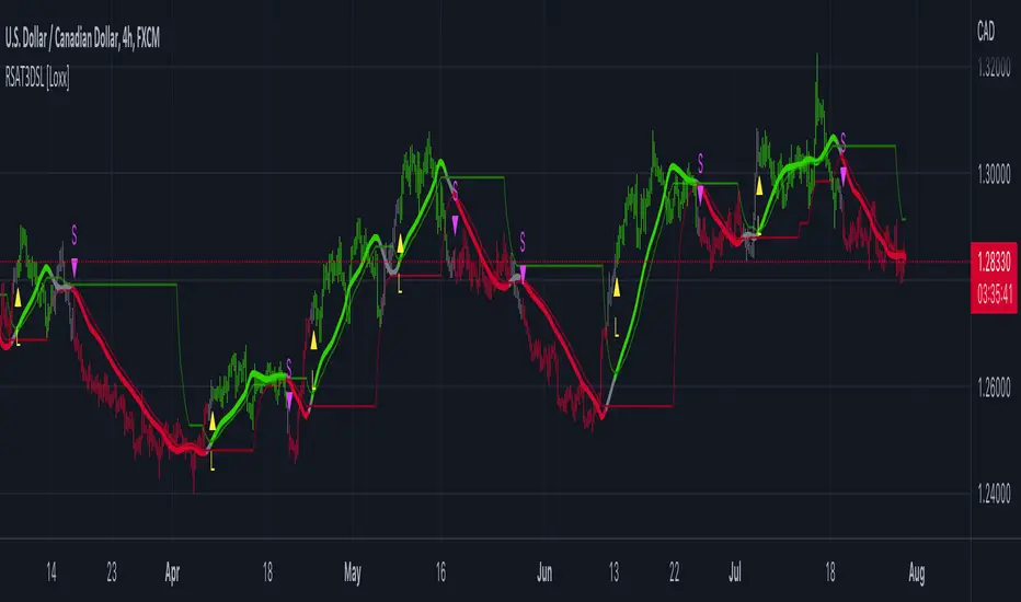
STD-Filterd, R-squared Adaptive T3 w/ Dynamic Zones [Loxx]STD-Filterd, R-squared Adaptive T3 w/ Dynamic Zones is a standard deviation filtered R-squared Adaptive T3 moving average with dynamic zones.
What is the T3 moving average?
Better Moving Averages Tim Tillson
November 1, 1998
Tim Tillson is a software project manager at Hewlett-Packard, with degrees in Mathematics and Computer Science. He has privately traded options and equities for 15 years.
Introduction
"Digital filtering includes the process of smoothing, predicting, differentiating, integrating, separation of signals, and removal of noise from a signal. Thus many people who do such things are actually using digital filters without realizing that they are; being unacquainted with the theory, they neither understand what they have done nor the possibilities of what they might have done."
This quote from R. W. Hamming applies to the vast majority of indicators in technical analysis . Moving averages, be they simple, weighted, or exponential, are lowpass filters; low frequency components in the signal pass through with little attenuation, while high frequencies are severely reduced.
"Oscillator" type indicators (such as MACD , Momentum, Relative Strength Index ) are another type of digital filter called a differentiator.
Tushar Chande has observed that many popular oscillators are highly correlated, which is sensible because they are trying to measure the rate of change of the underlying time series, i.e., are trying to be the first and second derivatives we all learned about in Calculus.
We use moving averages (lowpass filters) in technical analysis to remove the random noise from a time series, to discern the underlying trend or to determine prices at which we will take action. A perfect moving average would have two attributes:
It would be smooth, not sensitive to random noise in the underlying time series. Another way of saying this is that its derivative would not spuriously alternate between positive and negative values.
It would not lag behind the time series it is computed from. Lag, of course, produces late buy or sell signals that kill profits.
The only way one can compute a perfect moving average is to have knowledge of the future, and if we had that, we would buy one lottery ticket a week rather than trade!
Having said this, we can still improve on the conventional simple, weighted, or exponential moving averages. Here's how:
Two Interesting Moving Averages
We will examine two benchmark moving averages based on Linear Regression analysis.
In both cases, a Linear Regression line of length n is fitted to price data.
I call the first moving average ILRS, which stands for Integral of Linear Regression Slope. One simply integrates the slope of a linear regression line as it is successively fitted in a moving window of length n across the data, with the constant of integration being a simple moving average of the first n points. Put another way, the derivative of ILRS is the linear regression slope. Note that ILRS is not the same as a SMA ( simple moving average ) of length n, which is actually the midpoint of the linear regression line as it moves across the data.
We can measure the lag of moving averages with respect to a linear trend by computing how they behave when the input is a line with unit slope. Both SMA (n) and ILRS(n) have lag of n/2, but ILRS is much smoother than SMA .
Our second benchmark moving average is well known, called EPMA or End Point Moving Average. It is the endpoint of the linear regression line of length n as it is fitted across the data. EPMA hugs the data more closely than a simple or exponential moving average of the same length. The price we pay for this is that it is much noisier (less smooth) than ILRS, and it also has the annoying property that it overshoots the data when linear trends are present.
However, EPMA has a lag of 0 with respect to linear input! This makes sense because a linear regression line will fit linear input perfectly, and the endpoint of the LR line will be on the input line.
These two moving averages frame the tradeoffs that we are facing. On one extreme we have ILRS, which is very smooth and has considerable phase lag. EPMA has 0 phase lag, but is too noisy and overshoots. We would like to construct a better moving average which is as smooth as ILRS, but runs closer to where EPMA lies, without the overshoot.
A easy way to attempt this is to split the difference, i.e. use (ILRS(n)+EPMA(n))/2. This will give us a moving average (call it IE /2) which runs in between the two, has phase lag of n/4 but still inherits considerable noise from EPMA. IE /2 is inspirational, however. Can we build something that is comparable, but smoother? Figure 1 shows ILRS, EPMA, and IE /2.
Filter Techniques
Any thoughtful student of filter theory (or resolute experimenter) will have noticed that you can improve the smoothness of a filter by running it through itself multiple times, at the cost of increasing phase lag.
There is a complementary technique (called twicing by J.W. Tukey) which can be used to improve phase lag. If L stands for the operation of running data through a low pass filter, then twicing can be described by:
L' = L(time series) + L(time series - L(time series))
That is, we add a moving average of the difference between the input and the moving average to the moving average. This is algebraically equivalent to:
2L-L(L)
This is the Double Exponential Moving Average or DEMA , popularized by Patrick Mulloy in TASAC (January/February 1994).
In our taxonomy, DEMA has some phase lag (although it exponentially approaches 0) and is somewhat noisy, comparable to IE /2 indicator.
We will use these two techniques to construct our better moving average, after we explore the first one a little more closely.
Fixing Overshoot
An n-day EMA has smoothing constant alpha=2/(n+1) and a lag of (n-1)/2.
Thus EMA (3) has lag 1, and EMA (11) has lag 5. Figure 2 shows that, if I am willing to incur 5 days of lag, I get a smoother moving average if I run EMA (3) through itself 5 times than if I just take EMA (11) once.
This suggests that if EPMA and DEMA have 0 or low lag, why not run fast versions (eg DEMA (3)) through themselves many times to achieve a smooth result? The problem is that multiple runs though these filters increase their tendency to overshoot the data, giving an unusable result. This is because the amplitude response of DEMA and EPMA is greater than 1 at certain frequencies, giving a gain of much greater than 1 at these frequencies when run though themselves multiple times. Figure 3 shows DEMA (7) and EPMA(7) run through themselves 3 times. DEMA^3 has serious overshoot, and EPMA^3 is terrible.
The solution to the overshoot problem is to recall what we are doing with twicing:
DEMA (n) = EMA (n) + EMA (time series - EMA (n))
The second term is adding, in effect, a smooth version of the derivative to the EMA to achieve DEMA . The derivative term determines how hot the moving average's response to linear trends will be. We need to simply turn down the volume to achieve our basic building block:
EMA (n) + EMA (time series - EMA (n))*.7;
This is algebraically the same as:
EMA (n)*1.7-EMA( EMA (n))*.7;
I have chosen .7 as my volume factor, but the general formula (which I call "Generalized Dema") is:
GD (n,v) = EMA (n)*(1+v)-EMA( EMA (n))*v,
Where v ranges between 0 and 1. When v=0, GD is just an EMA , and when v=1, GD is DEMA . In between, GD is a cooler DEMA . By using a value for v less than 1 (I like .7), we cure the multiple DEMA overshoot problem, at the cost of accepting some additional phase delay. Now we can run GD through itself multiple times to define a new, smoother moving average T3 that does not overshoot the data:
T3(n) = GD ( GD ( GD (n)))
In filter theory parlance, T3 is a six-pole non-linear Kalman filter. Kalman filters are ones which use the error (in this case (time series - EMA (n)) to correct themselves. In Technical Analysis , these are called Adaptive Moving Averages; they track the time series more aggressively when it is making large moves.
What is R-squared Adaptive?
One tool available in forecasting the trendiness of the breakout is the coefficient of determination ( R-squared ), a statistical measurement.
The R-squared indicates linear strength between the security's price (the Y - axis) and time (the X - axis). The R-squared is the percentage of squared error that the linear regression can eliminate if it were used as the predictor instead of the mean value. If the R-squared were 0.99, then the linear regression would eliminate 99% of the error for prediction versus predicting closing prices using a simple moving average .
R-squared is used here to derive a T3 factor used to modify price before passing price through a six-pole non-linear Kalman filter.
What are Dynamic Zones?
As explained in "Stocks & Commodities V15:7 (306-310): Dynamic Zones by Leo Zamansky, Ph .D., and David Stendahl"
Most indicators use a fixed zone for buy and sell signals. Here’ s a concept based on zones that are responsive to past levels of the indicator.
One approach to active investing employs the use of oscillators to exploit tradable market trends. This investing style follows a very simple form of logic: Enter the market only when an oscillator has moved far above or below traditional trading lev- els. However, these oscillator- driven systems lack the ability to evolve with the market because they use fixed buy and sell zones. Traders typically use one set of buy and sell zones for a bull market and substantially different zones for a bear market. And therein lies the problem.
Once traders begin introducing their market opinions into trading equations, by changing the zones, they negate the system’s mechanical nature. The objective is to have a system automatically define its own buy and sell zones and thereby profitably trade in any market — bull or bear. Dynamic zones offer a solution to the problem of fixed buy and sell zones for any oscillator-driven system.
An indicator’s extreme levels can be quantified using statistical methods. These extreme levels are calculated for a certain period and serve as the buy and sell zones for a trading system. The repetition of this statistical process for every value of the indicator creates values that become the dynamic zones. The zones are calculated in such a way that the probability of the indicator value rising above, or falling below, the dynamic zones is equal to a given probability input set by the trader.
To better understand dynamic zones, let's first describe them mathematically and then explain their use. The dynamic zones definition:
Find V such that:
For dynamic zone buy: P{X <= V}=P1
For dynamic zone sell: P{X >= V}=P2
where P1 and P2 are the probabilities set by the trader, X is the value of the indicator for the selected period and V represents the value of the dynamic zone.
The probability input P1 and P2 can be adjusted by the trader to encompass as much or as little data as the trader would like. The smaller the probability, the fewer data values above and below the dynamic zones. This translates into a wider range between the buy and sell zones. If a 10% probability is used for P1 and P2, only those data values that make up the top 10% and bottom 10% for an indicator are used in the construction of the zones. Of the values, 80% will fall between the two extreme levels. Because dynamic zone levels are penetrated so infrequently, when this happens, traders know that the market has truly moved into overbought or oversold territory.
Calculating the Dynamic Zones
The algorithm for the dynamic zones is a series of steps. First, decide the value of the lookback period t. Next, decide the value of the probability Pbuy for buy zone and value of the probability Psell for the sell zone.
For i=1, to the last lookback period, build the distribution f(x) of the price during the lookback period i. Then find the value Vi1 such that the probability of the price less than or equal to Vi1 during the lookback period i is equal to Pbuy. Find the value Vi2 such that the probability of the price greater or equal to Vi2 during the lookback period i is equal to Psell. The sequence of Vi1 for all periods gives the buy zone. The sequence of Vi2 for all periods gives the sell zone.
In the algorithm description, we have: Build the distribution f(x) of the price during the lookback period i. The distribution here is empirical namely, how many times a given value of x appeared during the lookback period. The problem is to find such x that the probability of a price being greater or equal to x will be equal to a probability selected by the user. Probability is the area under the distribution curve. The task is to find such value of x that the area under the distribution curve to the right of x will be equal to the probability selected by the user. That x is the dynamic zone.
Included:
Bar coloring
Signals
Alerts
Loxx's Expanded Source Types

Pips-Stepped, R-squared Adaptive T3 [Loxx]Pips-Stepped, R-squared Adaptive T3 is a a T3 moving average with optional adaptivity, trend following, and pip-stepping. This indicator also uses optional flat coloring to determine chops zones. This indicator is R-squared adaptive. This is also an experimental indicator.
What is the T3 moving average?
Better Moving Averages Tim Tillson
November 1, 1998
Tim Tillson is a software project manager at Hewlett-Packard, with degrees in Mathematics and Computer Science. He has privately traded options and equities for 15 years.
Introduction
"Digital filtering includes the process of smoothing, predicting, differentiating, integrating, separation of signals, and removal of noise from a signal. Thus many people who do such things are actually using digital filters without realizing that they are; being unacquainted with the theory, they neither understand what they have done nor the possibilities of what they might have done."
This quote from R. W. Hamming applies to the vast majority of indicators in technical analysis . Moving averages, be they simple, weighted, or exponential, are lowpass filters; low frequency components in the signal pass through with little attenuation, while high frequencies are severely reduced.
"Oscillator" type indicators (such as MACD , Momentum, Relative Strength Index ) are another type of digital filter called a differentiator.
Tushar Chande has observed that many popular oscillators are highly correlated, which is sensible because they are trying to measure the rate of change of the underlying time series, i.e., are trying to be the first and second derivatives we all learned about in Calculus.
We use moving averages (lowpass filters) in technical analysis to remove the random noise from a time series, to discern the underlying trend or to determine prices at which we will take action. A perfect moving average would have two attributes:
It would be smooth, not sensitive to random noise in the underlying time series. Another way of saying this is that its derivative would not spuriously alternate between positive and negative values.
It would not lag behind the time series it is computed from. Lag, of course, produces late buy or sell signals that kill profits.
The only way one can compute a perfect moving average is to have knowledge of the future, and if we had that, we would buy one lottery ticket a week rather than trade!
Having said this, we can still improve on the conventional simple, weighted, or exponential moving averages. Here's how:
Two Interesting Moving Averages
We will examine two benchmark moving averages based on Linear Regression analysis.
In both cases, a Linear Regression line of length n is fitted to price data.
I call the first moving average ILRS, which stands for Integral of Linear Regression Slope. One simply integrates the slope of a linear regression line as it is successively fitted in a moving window of length n across the data, with the constant of integration being a simple moving average of the first n points. Put another way, the derivative of ILRS is the linear regression slope. Note that ILRS is not the same as a SMA ( simple moving average ) of length n, which is actually the midpoint of the linear regression line as it moves across the data.
We can measure the lag of moving averages with respect to a linear trend by computing how they behave when the input is a line with unit slope. Both SMA (n) and ILRS(n) have lag of n/2, but ILRS is much smoother than SMA .
Our second benchmark moving average is well known, called EPMA or End Point Moving Average. It is the endpoint of the linear regression line of length n as it is fitted across the data. EPMA hugs the data more closely than a simple or exponential moving average of the same length. The price we pay for this is that it is much noisier (less smooth) than ILRS, and it also has the annoying property that it overshoots the data when linear trends are present.
However, EPMA has a lag of 0 with respect to linear input! This makes sense because a linear regression line will fit linear input perfectly, and the endpoint of the LR line will be on the input line.
These two moving averages frame the tradeoffs that we are facing. On one extreme we have ILRS, which is very smooth and has considerable phase lag. EPMA has 0 phase lag, but is too noisy and overshoots. We would like to construct a better moving average which is as smooth as ILRS, but runs closer to where EPMA lies, without the overshoot.
A easy way to attempt this is to split the difference, i.e. use (ILRS(n)+EPMA(n))/2. This will give us a moving average (call it IE /2) which runs in between the two, has phase lag of n/4 but still inherits considerable noise from EPMA. IE /2 is inspirational, however. Can we build something that is comparable, but smoother? Figure 1 shows ILRS, EPMA, and IE /2.
Filter Techniques
Any thoughtful student of filter theory (or resolute experimenter) will have noticed that you can improve the smoothness of a filter by running it through itself multiple times, at the cost of increasing phase lag.
There is a complementary technique (called twicing by J.W. Tukey) which can be used to improve phase lag. If L stands for the operation of running data through a low pass filter, then twicing can be described by:
L' = L(time series) + L(time series - L(time series))
That is, we add a moving average of the difference between the input and the moving average to the moving average. This is algebraically equivalent to:
2L-L(L)
This is the Double Exponential Moving Average or DEMA , popularized by Patrick Mulloy in TASAC (January/February 1994).
In our taxonomy, DEMA has some phase lag (although it exponentially approaches 0) and is somewhat noisy, comparable to IE /2 indicator.
We will use these two techniques to construct our better moving average, after we explore the first one a little more closely.
Fixing Overshoot
An n-day EMA has smoothing constant alpha=2/(n+1) and a lag of (n-1)/2.
Thus EMA (3) has lag 1, and EMA (11) has lag 5. Figure 2 shows that, if I am willing to incur 5 days of lag, I get a smoother moving average if I run EMA (3) through itself 5 times than if I just take EMA (11) once.
This suggests that if EPMA and DEMA have 0 or low lag, why not run fast versions (eg DEMA (3)) through themselves many times to achieve a smooth result? The problem is that multiple runs though these filters increase their tendency to overshoot the data, giving an unusable result. This is because the amplitude response of DEMA and EPMA is greater than 1 at certain frequencies, giving a gain of much greater than 1 at these frequencies when run though themselves multiple times. Figure 3 shows DEMA (7) and EPMA(7) run through themselves 3 times. DEMA^3 has serious overshoot, and EPMA^3 is terrible.
The solution to the overshoot problem is to recall what we are doing with twicing:
DEMA (n) = EMA (n) + EMA (time series - EMA (n))
The second term is adding, in effect, a smooth version of the derivative to the EMA to achieve DEMA . The derivative term determines how hot the moving average's response to linear trends will be. We need to simply turn down the volume to achieve our basic building block:
EMA (n) + EMA (time series - EMA (n))*.7;
This is algebraically the same as:
EMA (n)*1.7-EMA( EMA (n))*.7;
I have chosen .7 as my volume factor, but the general formula (which I call "Generalized Dema") is:
GD (n,v) = EMA (n)*(1+v)-EMA( EMA (n))*v,
Where v ranges between 0 and 1. When v=0, GD is just an EMA , and when v=1, GD is DEMA . In between, GD is a cooler DEMA . By using a value for v less than 1 (I like .7), we cure the multiple DEMA overshoot problem, at the cost of accepting some additional phase delay. Now we can run GD through itself multiple times to define a new, smoother moving average T3 that does not overshoot the data:
T3(n) = GD ( GD ( GD (n)))
In filter theory parlance, T3 is a six-pole non-linear Kalman filter. Kalman filters are ones which use the error (in this case (time series - EMA (n)) to correct themselves. In Technical Analysis , these are called Adaptive Moving Averages; they track the time series more aggressively when it is making large moves.
What is R-squared Adaptive?
One tool available in forecasting the trendiness of the breakout is the coefficient of determination (R-squared), a statistical measurement.
The R-squared indicates linear strength between the security's price (the Y - axis) and time (the X - axis). The R-squared is the percentage of squared error that the linear regression can eliminate if it were used as the predictor instead of the mean value. If the R-squared were 0.99, then the linear regression would eliminate 99% of the error for prediction versus predicting closing prices using a simple moving average.
R-squared is used here to derive a T3 factor used to modify price before passing price through a six-pole non-linear Kalman filter.
Included:
Bar coloring
Signals
Alerts
Flat coloring
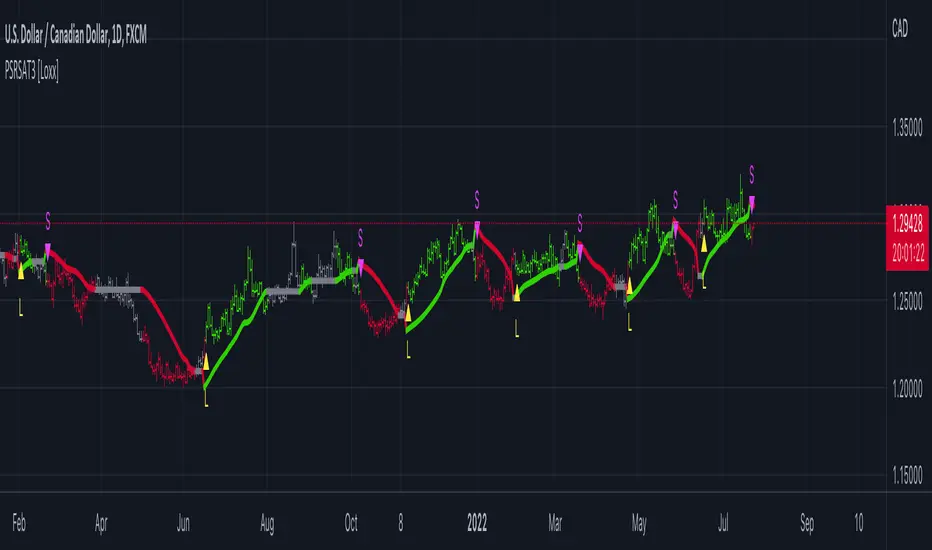
R-squared Adaptive T3 [Loxx]R-squared Adaptive T3 is an R-squared adaptive version of Tilson's T3 moving average. This adaptivity was originally proposed by mladen on various forex forums. This is considered experimental but shows how to use r-squared adapting methods to moving averages. In theory, the T3 is a six-pole non-linear Kalman filter.
What is the T3 moving average?
Better Moving Averages Tim Tillson
November 1, 1998
Tim Tillson is a software project manager at Hewlett-Packard, with degrees in Mathematics and Computer Science. He has privately traded options and equities for 15 years.
Introduction
"Digital filtering includes the process of smoothing, predicting, differentiating, integrating, separation of signals, and removal of noise from a signal. Thus many people who do such things are actually using digital filters without realizing that they are; being unacquainted with the theory, they neither understand what they have done nor the possibilities of what they might have done."
This quote from R. W. Hamming applies to the vast majority of indicators in technical analysis. Moving averages, be they simple, weighted, or exponential, are lowpass filters; low frequency components in the signal pass through with little attenuation, while high frequencies are severely reduced.
"Oscillator" type indicators (such as MACD, Momentum, Relative Strength Index) are another type of digital filter called a differentiator.
Tushar Chande has observed that many popular oscillators are highly correlated, which is sensible because they are trying to measure the rate of change of the underlying time series, i.e., are trying to be the first and second derivatives we all learned about in Calculus.
We use moving averages (lowpass filters) in technical analysis to remove the random noise from a time series, to discern the underlying trend or to determine prices at which we will take action. A perfect moving average would have two attributes:
It would be smooth, not sensitive to random noise in the underlying time series. Another way of saying this is that its derivative would not spuriously alternate between positive and negative values.
It would not lag behind the time series it is computed from. Lag, of course, produces late buy or sell signals that kill profits.
The only way one can compute a perfect moving average is to have knowledge of the future, and if we had that, we would buy one lottery ticket a week rather than trade!
Having said this, we can still improve on the conventional simple, weighted, or exponential moving averages. Here's how:
Two Interesting Moving Averages
We will examine two benchmark moving averages based on Linear Regression analysis.
In both cases, a Linear Regression line of length n is fitted to price data.
I call the first moving average ILRS, which stands for Integral of Linear Regression Slope. One simply integrates the slope of a linear regression line as it is successively fitted in a moving window of length n across the data, with the constant of integration being a simple moving average of the first n points. Put another way, the derivative of ILRS is the linear regression slope. Note that ILRS is not the same as a SMA (simple moving average) of length n, which is actually the midpoint of the linear regression line as it moves across the data.
We can measure the lag of moving averages with respect to a linear trend by computing how they behave when the input is a line with unit slope. Both SMA(n) and ILRS(n) have lag of n/2, but ILRS is much smoother than SMA.
Our second benchmark moving average is well known, called EPMA or End Point Moving Average. It is the endpoint of the linear regression line of length n as it is fitted across the data. EPMA hugs the data more closely than a simple or exponential moving average of the same length. The price we pay for this is that it is much noisier (less smooth) than ILRS, and it also has the annoying property that it overshoots the data when linear trends are present.
However, EPMA has a lag of 0 with respect to linear input! This makes sense because a linear regression line will fit linear input perfectly, and the endpoint of the LR line will be on the input line.
These two moving averages frame the tradeoffs that we are facing. On one extreme we have ILRS, which is very smooth and has considerable phase lag. EPMA has 0 phase lag, but is too noisy and overshoots. We would like to construct a better moving average which is as smooth as ILRS, but runs closer to where EPMA lies, without the overshoot.
A easy way to attempt this is to split the difference, i.e. use (ILRS(n)+EPMA(n))/2. This will give us a moving average (call it IE/2) which runs in between the two, has phase lag of n/4 but still inherits considerable noise from EPMA. IE/2 is inspirational, however. Can we build something that is comparable, but smoother? Figure 1 shows ILRS, EPMA, and IE/2.
Filter Techniques
Any thoughtful student of filter theory (or resolute experimenter) will have noticed that you can improve the smoothness of a filter by running it through itself multiple times, at the cost of increasing phase lag.
There is a complementary technique (called twicing by J.W. Tukey) which can be used to improve phase lag. If L stands for the operation of running data through a low pass filter, then twicing can be described by:
L' = L(time series) + L(time series - L(time series))
That is, we add a moving average of the difference between the input and the moving average to the moving average. This is algebraically equivalent to:
2L-L(L)
This is the Double Exponential Moving Average or DEMA, popularized by Patrick Mulloy in TASAC (January/February 1994).
In our taxonomy, DEMA has some phase lag (although it exponentially approaches 0) and is somewhat noisy, comparable to IE/2 indicator.
We will use these two techniques to construct our better moving average, after we explore the first one a little more closely.
Fixing Overshoot
An n-day EMA has smoothing constant alpha=2/(n+1) and a lag of (n-1)/2.
Thus EMA(3) has lag 1, and EMA(11) has lag 5. Figure 2 shows that, if I am willing to incur 5 days of lag, I get a smoother moving average if I run EMA(3) through itself 5 times than if I just take EMA(11) once.
This suggests that if EPMA and DEMA have 0 or low lag, why not run fast versions (eg DEMA(3)) through themselves many times to achieve a smooth result? The problem is that multiple runs though these filters increase their tendency to overshoot the data, giving an unusable result. This is because the amplitude response of DEMA and EPMA is greater than 1 at certain frequencies, giving a gain of much greater than 1 at these frequencies when run though themselves multiple times. Figure 3 shows DEMA(7) and EPMA(7) run through themselves 3 times. DEMA^3 has serious overshoot, and EPMA^3 is terrible.
The solution to the overshoot problem is to recall what we are doing with twicing:
DEMA(n) = EMA(n) + EMA(time series - EMA(n))
The second term is adding, in effect, a smooth version of the derivative to the EMA to achieve DEMA. The derivative term determines how hot the moving average's response to linear trends will be. We need to simply turn down the volume to achieve our basic building block:
EMA(n) + EMA(time series - EMA(n))*.7;
This is algebraically the same as:
EMA(n)*1.7-EMA(EMA(n))*.7;
I have chosen .7 as my volume factor, but the general formula (which I call "Generalized Dema") is:
GD(n,v) = EMA(n)*(1+v)-EMA(EMA(n))*v,
Where v ranges between 0 and 1. When v=0, GD is just an EMA, and when v=1, GD is DEMA. In between, GD is a cooler DEMA. By using a value for v less than 1 (I like .7), we cure the multiple DEMA overshoot problem, at the cost of accepting some additional phase delay. Now we can run GD through itself multiple times to define a new, smoother moving average T3 that does not overshoot the data:
T3(n) = GD(GD(GD(n)))
In filter theory parlance, T3 is a six-pole non-linear Kalman filter. Kalman filters are ones which use the error (in this case (time series - EMA(n)) to correct themselves. In Technical Analysis, these are called Adaptive Moving Averages; they track the time series more aggressively when it is making large moves.
Included:
Bar coloring
Signals
Alerts
Loxx's Expanded Source Types
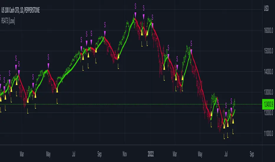
Multi-Indicator by johntradingwickThe Multi-Indicator includes the functionality of the following indicators:
1. Market Structure
2. Support and Resistance
3. VWAP
4. Simple Moving Average
5. Exponential Moving Average
Functionality of the Multi-Indicator:
Market Structure
As we already know, the market structure is one of the most important things in trading. If we are able to identify the trend correctly, it takes away a huge burden. For this, I have used the Zig Zag indicator to identify price trends. It plots points on the chart whenever the prices reverse by a larger percentage than a predetermined variable. The points are then connected by straight lines that will help you to identify the swing high and low.
This will help you to filter out any small price movements, making it easier to identify the trend, its direction, and its strength levels. You can change the period in consideration and the deviation by changing the deviation % and the depth.
Support and Resistance
The indicator provides the functionality to add support and resistance levels. If you want more levels just change the timeframe it looks at in the settings. It will pull the SR levels off the timeframe specified in the settings.
You can select the timeframe for support and resistance levels. The default time frame is “same as the chart”.
You can also extend lines to the right and change the width and colour of the lines. There is also an option to change the criteria to select the lines as valid support or resistance. You can extend the S/R level or use the horizontal lines to mark the level when there is a change in polarity.
VWAP
Volume Weighted Average Price (VWAP) is used to measure the average price weighted by volume. VWAP is typically used with intraday charts as a way to determine the general direction of intraday prices. It's similar to a moving average in that when the price is above VWAP, prices are rising and when the price is below VWAP, prices are falling. VWAP is primarily used by technical analysts to identify market trend.
Simple Moving Average
A simple Moving Average is an unweighted Moving Average. This means that each day in the data set has equal importance and is weighted equally. As each new day ends, the oldest data point is dropped and the newest one is added to the beginning.
The multi-indicator has the ability to provide 5 moving averages. This is particularly helpful if you want to use various time periods such as 20, 50, 100, and 200. Although this is just basic functionality, it comes in handy if you are using a free account.
Exponential Moving Average
An exponential moving average (EMA) is a type of moving average (MA) that places a greater weight and significance on the most recent data points. An exponentially weighted moving average reacts more significantly to recent price changes than a simple moving average. The multi-indicator provides 5 exponential moving averages. This is particularly helpful if you want to use various time periods such as 20, 50, 100, and 200.
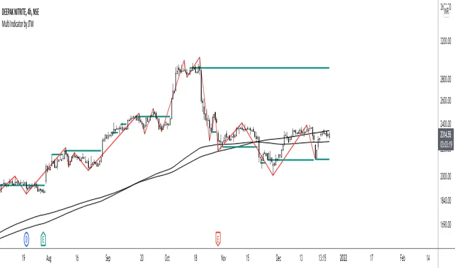
paigep.llc - SuperMA
SuperMA is a multi-layered moving-average and candle-coloring system that combines SMA, EMA, and optional HMA logic to help traders visualize trend shifts, pullbacks, and momentum changes in a clean, structured way.
The script includes multiple modules: trend-based moving averages, pullback signals, exit logic, and an optional HMA cross engine.
📌 Core Features
1. Full SMA + EMA Framework
The indicator plots multiple moving averages (8, 9, 13, 20, 50, 200) using both SMA and EMA calculations. Each line automatically colors bullish or bearish based on its relationship to the 200-period baseline. Users can toggle SMAs and EMAs independently for clearer chart control.
2. Main Trend Entry & Exit Logic (8×200 and 8×20)
Built-in crossover logic detects:
Main Entry: SMA 8 crossing above/below EMA 200
Main Exit: SMA 8 and SMA 20 cross (with an option to choose which SMA is treated as the “fast” leg)
A “first exit only” option allows the script to ignore additional exit signals until a new trend regime begins.
3. Pullback Module (20 SMA Interaction)
Pullback entries and exits occur when price crosses the 20 SMA during existing trend conditions.
This includes:
Pullback entries through the 20 SMA
Pullback exits back across the 20 SMA
Labels and candle colors are available for all pullback events.
4. Optional HMA Cross Module
A separate module allows traders to use two Hull Moving Averages (HMA) with customizable:
Lengths
Independent timeframes
Line colors
Cross-based entries and exits
This module has its own events, labels, and optional candle coloring.
5. Advanced Candle Coloring System
Candle coloring is layered in priority order, based on:
Main trend entries
Main exits
HMA entries
HMA exits
Pullback entries
Pullback exits
Trend-only candles (based on SMA 8 relative to EMA 200)
Users may also independently color wicks and borders.
6. Configurable Alerts (Fully Decoupled from Visuals)
Alerts are available for all major events, including:
Main Entries (8×200)
Main Exits (8×20)
Pullback Entries and Exits
HMA Entries and Exits
Bull or Bear Trend candles
Any colored candle event
Alerts can fire on bar close only or intrabar, depending on user preference.
Use Cases
SuperMA helps traders visualize:
Trend direction using SMA/EMA structure
Momentum shifts through HMA crosses
Pullback zones around the 20 SMA
Early regime transitions based on the 8×200 relationship
Candle-level context through color-coded bars
The indicator works across all markets and timeframes.
⚠️ Note
This tool is for visual and analytical assistance only. It does not guarantee future performance and should be combined with additional analysis and risk management.
