Reversal WaveThis is the type of quantitative system that can get you hated on investment forums, now that the Random Walk Theory is back in fashion. The strategy has simple price action rules, zero over-optimization, and is validated by a historical record of nearly a century on both Gold and the S&P 500 index.
Recommended Markets
SPX (Weekly, Monthly)
SPY (Monthly)
Tesla (Weekly)
XAUUSD (Weekly, Monthly)
NVDA (Weekly, Monthly)
Meta (Weekly, Monthly)
GOOG (Weekly, Monthly)
MSFT (Weekly, Monthly)
AAPL (Weekly, Monthly)
System Rules and Parameters
Total capital: $10,000
We will use 10% of the total capital per trade
Commissions will be 0.1% per trade
Condition 1: Previous Bearish Candle (isPrevBearish) (the closing price was lower than the opening price).
Condition 2: Midpoint of the Body The script calculates the exact midpoint of the body of that previous bearish candle.
• Formula: (Previous Open + Previous Close) / 2.
Condition 3: 50% Recovery (longCondition) The current candle must be bullish (green) and, most importantly, its closing price must be above the midpoint calculated in the previous step.
Once these parameters are met, the system executes a long entry and calculates the exit parameters:
Stop Loss (SL): Placed at the low of the candle that generated the entry signal.
Take Profit (TP): Calculated by projecting the risk distance upward.
• Calculation: Entry Price + (Risk * 1).
Risk:Reward Ratio of 1:1.
About the Profit Factor
In my experience, TradingView calculates profits and losses based on the percentage of movement, which can cause returns to not match expectations. This doesn’t significantly affect trending systems, but it can impact systems with a high win rate and a well-defined risk-reward ratio. It only takes one large entry candle that triggers the SL to translate into a major drop in performance.
For example, you might see a system with a 60% win rate and a 1:1 risk-reward ratio generating losses, even though commissions are under control relative to the number of trades.
My recommendation is to manually calculate the performance of systems with a well-defined risk-reward ratio, assuming you will trade using a fixed amount per trade and limit losses to a fixed percentage.
Remember that, even if candles are larger or smaller in size, we can maintain a fixed loss percentage by using leverage (in cases of low volatility) or reducing the capital at risk (when volatility is high).
Implementing leverage or capital reduction based on volatility is something I haven’t been able to incorporate into the code, but it would undoubtedly improve the system’s performance dramatically, as it would fix a consistent loss percentage per trade, preventing losses from fluctuating with volatility swings.
For example, we can maintain a fixed loss percentage when volatility is low by using the following formula:
Leverage = % of SL you’re willing to risk / % volatility from entry point to exit or SL
And if volatility is high and exceeds the fixed percentage we want to expose per trade (if SL is hit), we could reduce the position size.
For example, imagine we only want to risk 15% per SL on Tesla, where volatility is high and would cause a 23.57% loss. In this case, we subtract 23.57% from 15% (the loss percentage we’re willing to accept per trade), then subtract the result from our usual position size.
23.57% - 15% = 8.57%
Suppose I use $200 per trade.
To calculate 8.57% of $200, simply multiply 200 by 8.57/100. This simple calculation shows that 8.57% equals about $17.14 of the $200. Then subtract that value from $200:
$200 - $17.14 = $182.86
In summary, if we reduced the position size to $182.86 (from the usual $200, where we’re willing to lose 15%), no matter whether Tesla moves up or down 23.57%, we would still only gain or lose 15% of the $200, thus respecting our risk management.
Final Notes
The code is extremely simple, and every step of its development is detailed within it.
If you liked this strategy, which complements very well with others I’ve already published, stay tuned. Best regards.
Tìm kiếm tập lệnh với "META股价历史数据"

Vital Wave 20-50Simplicity is almost always the most effective approach, and here I’m giving you a trend-following system that exploits the bullish bias of traditional markets and their trending nature, with very basic rules.
Rules (long entries only)
• Market entry: When the EMA 20 crosses above the EMA 50 (from below)
• Main market exit: When the EMA 20 crosses below the EMA 50 (from above)
• Fixed Stop Loss: Placed at the price level of the Lower Bollinger Band at the moment the trade is entered.
In my strategy, the primary exit is when the EMA 20 crosses below the EMA 50. However, this crossover can sometimes take a while to occur, and in the meantime the price may have already dropped significantly. The Stop Loss based on the Lower Bollinger Band is designed to limit losses in case the market moves sharply against the position without giving the bearish crossover signal in time. Having two exit conditions makes the strategy much more robust in terms of risk management.
Risk Management:
• Initial capital: $10,000
• Position size: 10% of available capital per trade
• Commissions: 0.1% on traded volume
• Stop Loss: Based on the Lower Bollinger Band
• Take Profit / Exit: When EMA 20 crosses below EMA 50
Recommended Markets:
XAUUSD (OANDA) (Daily)
Period: January 3, 1833 – November 23, 2025
Total Profit & Loss: +$6,030.62 USD (+57.57%)
Maximum Drawdown: $541.53 USD (3.83%)
Total Trades: 136
Winning Trades (Win Rate): 36.03% (49/136)
Profit Factor: 2.483
XAUUSD (OANDA) (12-hour)
Period: March 19, 2006 – November 23, 2025
Total Profit & Loss: +$1,209.56 USD (+11.89%)
Maximum Drawdown: $384.58 USD (3.61%)
Total Trades: 97
Winning Trades (Win Rate): 35.05% (34/97)
Profit Factor: 1.676
XAUUSD (OANDA) (8-hour)
Period: March 19, 2006 – November 23, 2025
Total Profit & Loss: +$1,179.36 USD (+11.81%)
Maximum Drawdown: $246.88 USD (2.32%)
Total Trades: 147
Winning Trades (Win Rate): 31.97% (47/147)
Profit Factor: 1.626
Tesla (NASDAQ) (4-hour)
Period: June 29, 2010 – November 23, 2025
Total Profit & Loss (Absolute): +$11,687.90 USD (+116.88%)
Maximum Drawdown: $922.05 USD (6.50%)
Total Trades: 68
Winning Trades (Win Rate): 39.71% (27/68)
Profit Factor: 4.156
Tesla (NASDAQ) (3-hour)
Total Profit & Loss: +$11,522.33 USD (+115.22%)
Maximum Drawdown: $1,247.60 USD (8.80%)
Total Trades: 114
Winning Trades: 33.33% (38/114)
Profit Factor: 2.811
Additional Recommendations
(These assets have shown good trending behavior with the same strategy across multiple timeframes):
• NVDA (15 min, 30 min, 1h, 2h, 3h, 4h, 6h, 8h, 12h, Daily)
• NFLX (1h, 2h, 3h, 4h, 6h, 8h, 12h, Daily)
• MA (1h, 2h, 3h, 4h, 6h, 8h, 12h, Daily)
• META (1h, 2h, 3h, 4h, 6h, 8h, 12h, Daily)
• AAPL (1h, 2h, 3h, 4h, 6h, 8h, 12h, Daily)
• SPY (12h, Daily)
About the Code
The user can modify:
• EMA periods (20 and 50 by default)
• Bollinger Bands length (20 periods)
• Standard deviation (2.0)
Visualization
• EMA 20: Blue line
• EMA 50: Red line
• Green background when EMA20 > EMA50 (bullish trend)
• Red background when EMA20 < EMA50 (bearish trend)
Important Note:
We can significantly increase the profit factor and overall profitability by risking a fixed percentage per trade instead of a fixed amount. This would prevent losses from fluctuating with changes in volatility.
This could be implemented by reducing position size or adjusting leverage based on the volatility percentage required for each trade, but I’m not sure if this is fully possible in Pine Script. In my other script, “ Golden Cross 50/200 EMA ,” I go deeper into this topic and provide examples.
I hope you enjoy this contribution. Best regards!

Golden Cross 50/200 EMATrend-following systems are characterized by having a low win rate, yet in the right circumstances (trending markets and higher timeframes) they can deliver returns that even surpass those of systems with a high win rate.
Below, I show you a simple bullish trend-following system with clear execution rules:
System Rules
-Long entries when the 50-period EMA crosses above the 200-period EMA.
-Stop Loss (SL) placed at the lowest low of the 15 candles prior to the entry candle.
-Take Profit (TP) triggered when the 50-period EMA crosses below the 200-period EMA.
Risk Management
-Initial capital: $10,000
-Position size: 10% of capital per trade
-Commissions: 0.1% per trade
Important Note:
In the code, the stop loss is defined using the swing low (15 candles), but the position size is not adjusted based on the distance to the stop loss. In other words, 10% of the equity is risked on each trade, but the actual loss on the trade is not controlled by a maximum fixed percentage of the account — it depends entirely on the stop loss level. This means the loss on a single trade could be significantly higher or lower than 10% of the account equity, depending on volatility.
Implementing leverage or reducing position size based on volatility is something I haven’t been able to include in the code, but it would dramatically improve the system’s performance. It would fix a consistent percentage loss per trade, preventing losses from fluctuating wildly with changes in volatility.
For example, we can maintain a fixed loss percentage when volatility is low by using the following formula:
Leverage = % of SL you’re willing to risk / % volatility from entry point to stop loss
And when volatility is high and would exceed the fixed percentage we want to expose per trade (if the SL is hit), we could reduce the position size accordingly.
Practical example:
Imagine we only want to risk 15% of the position value if the stop loss is triggered on Tesla (which has high volatility), but the distance to the SL represents a potential 23.57% drop. In this case, we subtract the desired risk (15%) from the actual volatility-based loss (23.57%):
23.57% − 15% = 8.57%
Now suppose we normally use $200 per trade.
To calculate 8.57% of $200:
200 × (8.57 / 100) = $17.14
Then subtract that amount from the original position size:
$200 − $17.14 = $182.86
In summary:
If we reduce the position size to $182.86 (instead of the usual $200), even if Tesla moves 23.57% against us and hits the stop loss, we would still only lose approximately 15% of the original $200 position — exactly the risk level we defined. This way, we strictly respect our risk management rules regardless of volatility swings.
I hope this clearly explains the importance of capping losses at a fixed percentage per trade. This keeps risk under control while maintaining a consistent percentage of capital invested per trade — preventing both statistical distortion of the system and the potential destruction of the account.
About the code:
Strategy declaration:
The strategy is named 'Golden Cross 50/200 EMA'.
overlay=true means it will be drawn directly on the price chart.
initial_capital=10000 sets the initial capital to $10,000.
default_qty_type=strategy.percent_of_equity and default_qty_value=10 means each trade uses 10% of available equity.
margin_long=0 indicates no margin is used for long positions (this is likely for simulation purposes only; in real trading, margin would be required).
commission_type=strategy.commission.percent and commission_value=0.1 sets a 0.1% commission per trade.
Indicators:
Calculates two EMAs: a 50-period EMA (ema50) and a 200-period EMA (ema200).
Crossover detection:
bullCross is triggered when the 50-period EMA crosses above the 200-period EMA (Golden Cross).
bearCross is triggered when the 50-period EMA crosses below the 200-period EMA (Death Cross).
Recent swing:
swingLow calculates the lowest low of the previous 15 periods.
Stop Loss:
entryStopLoss is a variable initialized as na (not available) and is updated to the current swingLow value whenever a bullCross occurs.
Entry and exit conditions:
Entry: When a bullCross occurs, the initial stop loss is set to the current swingLow and a long position is opened.
Exit on opposite signal: When a bearCross occurs, the long position is closed.
Exit on stop loss: If the price falls below entryStopLoss while a position is open, the position is closed.
Visualization:
Both EMAs are plotted (50-period in blue, 200-period in red).
Green triangles are plotted below the bar on a bullCross, and red triangles above the bar on a bearCross.
A horizontal orange line is drawn that shows the stop loss level whenever a position is open.
Alerts:
Alerts are created for:Long entry
Exit on bearish crossover (Death Cross)
Exit triggered by stop loss
Favorable Conditions:
Tesla (45-minute timeframe)
June 29, 2010 – November 17, 2025
Total net profit: $12,458.73 or +124.59%
Maximum drawdown: $1,210.40 or 8.29%
Total trades: 107
Winning trades: 27.10% (29/107)
Profit factor: 3.141
Tesla (1-hour timeframe)
June 29, 2010 – November 17, 2025
Total net profit: $7,681.83 or +76.82%
Maximum drawdown: $993.36 or 7.30%
Total trades: 75
Winning trades: 29.33% (22/75)
Profit factor: 3.157
Netflix (45-minute timeframe)
May 23, 2002 – November 17, 2025
Total net profit: $11,380.73 or +113.81%
Maximum drawdown: $699.45 or 5.98%
Total trades: 134
Winning trades: 36.57% (49/134)
Profit factor: 2.885
Netflix (1-hour timeframe)
May 23, 2002 – November 17, 2025
Total net profit: $11,689.05 or +116.89%
Maximum drawdown: $844.55 or 7.24%
Total trades: 107
Winning trades: 37.38% (40/107)
Profit factor: 2.915
Netflix (2-hour timeframe)
May 23, 2002 – November 17, 2025
Total net profit: $12,807.71 or +128.10%
Maximum drawdown: $866.52 or 6.03%
Total trades: 56
Winning trades: 41.07% (23/56)
Profit factor: 3.891
Meta (45-minute timeframe)
May 18, 2012 – November 17, 2025
Total net profit: $2,370.02 or +23.70%
Maximum drawdown: $365.27 or 3.50%
Total trades: 83
Winning trades: 31.33% (26/83)
Profit factor: 2.419
Apple (45-minute timeframe)
January 3, 2000 – November 17, 2025
Total net profit: $8,232.55 or +80.59%
Maximum drawdown: $581.11 or 3.16%
Total trades: 140
Winning trades: 34.29% (48/140)
Profit factor: 3.009
Apple (1-hour timeframe)
January 3, 2000 – November 17, 2025
Total net profit: $9,685.89 or +94.93%
Maximum drawdown: $374.69 or 2.26%
Total trades: 118
Winning trades: 35.59% (42/118)
Profit factor: 3.463
Apple (2-hour timeframe)
January 3, 2000 – November 17, 2025
Total net profit: $8,001.28 or +77.99%
Maximum drawdown: $755.84 or 7.56%
Total trades: 67
Winning trades: 41.79% (28/67)
Profit factor: 3.825
NVDA (15-minute timeframe)
January 3, 2000 – November 17, 2025
Total net profit: $11,828.56 or +118.29%
Maximum drawdown: $1,275.43 or 8.06%
Total trades: 466
Winning trades: 28.11% (131/466)
Profit factor: 2.033
NVDA (30-minute timeframe)
January 3, 2000 – November 17, 2025
Total net profit: $12,203.21 or +122.03%
Maximum drawdown: $1,661.86 or 10.35%
Total trades: 245
Winning trades: 28.98% (71/245)
Profit factor: 2.291
NVDA (45-minute timeframe)
January 3, 2000 – November 17, 2025
Total net profit: $16,793.48 or +167.93%
Maximum drawdown: $1,458.81 or 8.40%
Total trades: 172
Winning trades: 33.14% (57/172)
Profit factor: 2.927

ECG PRICE - mauricioofsousa📉 ECG PRICE – The Price Electrocardiogram
(explained for traders, scientists, and complete beginners)
🔍 1. WHAT IS THE ECG PRICE?
The ECG PRICE protocol is a market-reading system based on the RSI, but with a surgical twist:
👉 You don’t just calculate RSI from price.
👉 You adjust the price using the RSI, and then calculate RSI over this adjusted price.
This creates a filtered, amplified signal that behaves like a heart monitor for price, detecting micro-impulses and subtle market movements long before they show up in the standard RSI.
🧬 2. CORE IDEA
Just like a real ECG amplifies and reveals electrical rhythms hidden inside the heartbeat,
the ECG PRICE amplifies micro-deformations hidden inside the price’s momentum.
It works in three stages:
Compute the regular RSI
Use the RSI to adjust the price (creating an electrocardiographic price)
Compute a second RSI over this modified price
The result is a meta-derived oscillator—more sensitive, more precise, and better at detecting structural changes.
🧩 3. TECHNICAL BREAKDOWN
3.1. First RSI (classic)
The script calculates:
average gains
average losses
relative strength (RS)
and then the standard 0–100 RSI
This is the “normal heart rate monitor” everyone uses.
3.2. Creating the “Adjusted Price”
adjustedPrice = close * (rsi / 100)
This means:
➡️ When RSI is high (strong buying momentum), price is amplified.
➡️ When RSI is low (strong selling momentum), price is compressed.
This converts raw price into a bio-electrical signal, where the price itself is modulated by its own internal momentum.
It’s the financial equivalent of ECG gain adjustment.
3.3. RSI of the Adjusted Price
Now the script calculates a new RSI from this modified price.
That is the actual ECG PRICE.
This second-order oscillator becomes extremely sensitive to:
micro-momentum shifts
early trend fading
volatility shocks
micro-divergences
institutional pressure waves
It reads the electrical pattern behind the price rather than the superficial movement.
🟩🟥 4. Diagnostic Lines of the Protocol
35 (green dotted)
Pre-oversold fatigue zone.
65 (red dotted)
Pre-overbought exhaustion zone.
30 (white solid)
Classic oversold.
70 (white solid)
Classic overbought.
Together they create two diagnostic corridors:
1. Medical corridor (30–70):
Standard RSI clinical range.
2. Electrical corridor (35–65):
The ECG-sensitive zone where micro-shifts appear first.
🧠 5. In Engineering Language (MGO style)
The ECG PRICE is essentially:
A nonlinear second-order oscillator where the RSI feeds back into price, creating a recursive momentum-modulated signal.
It functions like a:
bioinformational modulator
feedback-driven wave processor
impulse amplifier
micro-PID sensitivity enhancer
Very similar to the informational-wave transformations inside the MGO pipeline.
👨⚕️📉 6. Explained for a Total Beginner
Imagine the price is a heart.
The normal RSI shows if the heart is beating fast or slow.
But the ECG PRICE takes that heartbeat…
feeds it back into the heart…
and then measures the new heartbeat.
This creates a much more sensitive exam that detects problems before the normal test would.
💡 7. What It Gives You in Practice
earlier reversal signals
better trend-fatigue detection
clearer micro-divergences
a clean RSI with reduced noise
a smoother momentum curve
advanced behavioral readings before breakouts
It’s an upgrade.
A second-layer RSI that “hears” the inner electrical impulses of price.

Algorithm Predator - ML-liteAlgorithm Predator - ML-lite
This indicator combines four specialized trading agents with an adaptive multi-armed bandit selection system to identify high-probability trade setups. It is designed for swing and intraday traders who want systematic signal generation based on institutional order flow patterns , momentum exhaustion , liquidity dynamics , and statistical mean reversion .
Core Architecture
Why These Components Are Combined:
The script addresses a fundamental challenge in algorithmic trading: no single detection method works consistently across all market conditions. By deploying four independent agents and using reinforcement learning algorithms to select or blend their outputs, the system adapts to changing market regimes without manual intervention.
The Four Trading Agents
1. Spoofing Detector Agent 🎭
Detects iceberg orders through persistent volume at similar price levels over 5 bars
Identifies spoofing patterns via asymmetric wick analysis (wicks exceeding 60% of bar range with volume >1.8× average)
Monitors order clustering using simplified Hawkes process intensity tracking (exponential decay model)
Signal Logic: Contrarian—fades false breakouts caused by institutional manipulation
Best Markets: Consolidations, institutional trading windows, low-liquidity hours
2. Exhaustion Detector Agent ⚡
Calculates RSI divergence between price movement and momentum indicator over 5-bar window
Detects VWAP exhaustion (price at 2σ bands with declining volume)
Uses VPIN reversals (volume-based toxic flow dissipation) to identify momentum failure
Signal Logic: Counter-trend—enters when momentum extreme shows weakness
Best Markets: Trending markets reaching climax points, over-extended moves
3. Liquidity Void Detector Agent 💧
Measures Bollinger Band squeeze (width <60% of 50-period average)
Identifies stop hunts via 20-bar high/low penetration with immediate reversal and volume spike
Detects hidden liquidity absorption (volume >2× average with range <0.3× ATR)
Signal Logic: Breakout anticipation—enters after liquidity grab but before main move
Best Markets: Range-bound pre-breakout, volatility compression zones
4. Mean Reversion Agent 📊
Calculates price z-scores relative to 50-period SMA and standard deviation (triggers at ±2σ)
Implements Ornstein-Uhlenbeck process scoring (mean-reverting stochastic model)
Uses entropy analysis to detect algorithmic trading patterns (low entropy <0.25 = high predictability)
Signal Logic: Statistical reversion—enters when price deviates significantly from statistical equilibrium
Best Markets: Range-bound, low-volatility, algorithmically-dominated instruments
Adaptive Selection: Multi-Armed Bandit System
The script implements four reinforcement learning algorithms to dynamically select or blend agents based on performance:
Thompson Sampling (Default - Recommended):
Uses Bayesian inference with beta distributions (tracks alpha/beta parameters per agent)
Balances exploration (trying underused agents) vs. exploitation (using proven winners)
Each agent's win/loss history informs its selection probability
Lite Approximation: Uses pseudo-random sampling from price/volume noise instead of true random number generation
UCB1 (Upper Confidence Bound):
Calculates confidence intervals using: average_reward + sqrt(2 × ln(total_pulls) / agent_pulls)
Deterministic algorithm favoring agents with high uncertainty (potential upside)
More conservative than Thompson Sampling
Epsilon-Greedy:
Exploits best-performing agent (1-ε)% of the time
Explores randomly ε% of the time (default 10%, configurable 1-50%)
Simple, transparent, easily tuned via epsilon parameter
Gradient Bandit:
Uses softmax probability distribution over agent preference weights
Updates weights via gradient ascent based on rewards
Best for Blend mode where all agents contribute
Selection Modes:
Switch Mode: Uses only the selected agent's signal (clean, decisive)
Blend Mode: Combines all agents using exponentially weighted confidence scores controlled by temperature parameter (smooth, diversified)
Lock Agent Feature:
Optional manual override to force one specific agent
Useful after identifying which agent dominates your specific instrument
Only applies in Switch mode
Four choices: Spoofing Detector, Exhaustion Detector, Liquidity Void, Mean Reversion
Memory System
Dual-Layer Architecture:
Short-Term Memory: Stores last 20 trade outcomes per agent (configurable 10-50)
Long-Term Memory: Stores episode averages when short-term reaches transfer threshold (configurable 5-20 bars)
Memory Boost Mechanism: Recent performance modulates agent scores by up to ±20%
Episode Transfer: When an agent accumulates sufficient results, averages are condensed into long-term storage
Persistence: Manual restoration of learned parameters via input fields (alpha, beta, weights, microstructure thresholds)
How Memory Works:
Agent generates signal → outcome tracked after 8 bars (performance horizon)
Result stored in short-term memory (win = 1.0, loss = 0.0)
Short-term average influences agent's future scores (positive feedback loop)
After threshold met (default 10 results), episode averaged into long-term storage
Long-term patterns (weighted 30%) + short-term patterns (weighted 70%) = total memory boost
Market Microstructure Analysis
These advanced metrics quantify institutional order flow dynamics:
Order Flow Toxicity (Simplified VPIN):
Measures buy/sell volume imbalance over 20 bars: |buy_vol - sell_vol| / (buy_vol + sell_vol)
Detects informed trading activity (institutional players with non-public information)
Values >0.4 indicate "toxic flow" (informed traders active)
Lite Approximation: Uses simple open/close heuristic instead of tick-by-tick trade classification
Price Impact Analysis (Simplified Kyle's Lambda):
Measures market impact efficiency: |price_change_10| / sqrt(volume_sum_10)
Low values = large orders with minimal price impact ( stealth accumulation )
High values = retail-dominated moves with high slippage
Lite Approximation: Uses simplified denominator instead of regression-based signed order flow
Market Randomness (Entropy Analysis):
Counts unique price changes over 20 bars / 20
Measures market predictability
High entropy (>0.6) = human-driven, chaotic price action
Low entropy (<0.25) = algorithmic trading dominance (predictable patterns)
Lite Approximation: Simple ratio instead of true Shannon entropy H(X) = -Σ p(x)·log₂(p(x))
Order Clustering (Simplified Hawkes Process):
Tracks self-exciting event intensity (coordinated order activity)
Decays at 0.9× per bar, spikes +1.0 when volume >1.5× average
High intensity (>0.7) indicates clustering (potential spoofing/accumulation)
Lite Approximation: Simple exponential decay instead of full λ(t) = μ + Σ α·exp(-β(t-tᵢ)) with MLE
Signal Generation Process
Multi-Stage Validation:
Stage 1: Agent Scoring
Each agent calculates internal score based on its detection criteria
Scores must exceed agent-specific threshold (adjusted by sensitivity multiplier)
Agent outputs: Signal direction (+1/-1/0) and Confidence level (0.0-1.0)
Stage 2: Memory Boost
Agent scores multiplied by memory boost factor (0.8-1.2 based on recent performance)
Successful agents get amplified, failing agents get dampened
Stage 3: Bandit Selection/Blending
If Adaptive Mode ON:
Switch: Bandit selects single best agent, uses only its signal
Blend: All agents combined using softmax-weighted confidence scores
If Adaptive Mode OFF:
Traditional consensus voting with confidence-squared weighting
Signal fires when consensus exceeds threshold (default 70%)
Stage 4: Confirmation Filter
Raw signal must repeat for consecutive bars (default 3, configurable 2-4)
Minimum confidence threshold: 0.25 (25%) enforced regardless of mode
Trend alignment check: Long signals require trend_score ≥ -2, Short signals require trend_score ≤ 2
Stage 5: Cooldown Enforcement
Minimum bars between signals (default 10, configurable 5-15)
Prevents over-trading during choppy conditions
Stage 6: Performance Tracking
After 8 bars (performance horizon), signal outcome evaluated
Win = price moved in signal direction, Loss = price moved against
Results fed back into memory and bandit statistics
Trading Modes (Presets)
Pre-configured parameter sets:
Conservative: 85% consensus, 4 confirmations, 15-bar cooldown
Expected: 60-70% win rate, 3-8 signals/week
Best for: Swing trading, capital preservation, beginners
Balanced: 70% consensus, 3 confirmations, 10-bar cooldown
Expected: 55-65% win rate, 8-15 signals/week
Best for: Day trading, most traders, general use
Aggressive: 60% consensus, 2 confirmations, 5-bar cooldown
Expected: 50-58% win rate, 15-30 signals/week
Best for: Scalping, high-frequency trading, active management
Elite: 75% consensus, 3 confirmations, 12-bar cooldown
Expected: 58-68% win rate, 5-12 signals/week
Best for: Selective trading, high-conviction setups
Adaptive: 65% consensus, 2 confirmations, 8-bar cooldown
Expected: Varies based on learning
Best for: Experienced users leveraging bandit system
How to Use
1. Initial Setup (5 Minutes):
Select Trading Mode matching your style (start with Balanced)
Enable Adaptive Learning (recommended for automatic agent selection)
Choose Thompson Sampling algorithm (best all-around performance)
Keep Microstructure Metrics enabled for liquid instruments (>100k daily volume)
2. Agent Tuning (Optional):
Adjust Agent Sensitivity multipliers (0.5-2.0):
<0.8 = Highly selective (fewer signals, higher quality)
0.9-1.2 = Balanced (recommended starting point)
1.3 = Aggressive (more signals, lower individual quality)
Monitor dashboard for 20-30 signals to identify dominant agent
If one agent consistently outperforms, consider using Lock Agent feature
3. Bandit Configuration (Advanced):
Blend Temperature (0.1-2.0):
0.3 = Sharp decisions (best agent dominates)
0.5 = Balanced (default)
1.0+ = Smooth (equal weighting, democratic)
Memory Decay (0.8-0.99):
0.90 = Fast adaptation (volatile markets)
0.95 = Balanced (most instruments)
0.97+ = Long memory (stable trends)
4. Signal Interpretation:
Green triangle (▲): Long signal confirmed
Red triangle (▼): Short signal confirmed
Dashboard shows:
Active agent (highlighted row with ► marker)
Win rate per agent (green >60%, yellow 40-60%, red <40%)
Confidence bars (█████ = maximum confidence)
Memory size (short-term buffer count)
Colored zones display:
Entry level (current close)
Stop-loss (1.5× ATR)
Take-profit 1 (2.0× ATR)
Take-profit 2 (3.5× ATR)
5. Risk Management:
Never risk >1-2% per signal (use ATR-based stops)
Signals are entry triggers, not complete strategies
Combine with your own market context analysis
Consider fundamental catalysts and news events
Use "Confirming" status to prepare entries (not to enter early)
6. Memory Persistence (Optional):
After 50-100 trades, check Memory Export Panel
Record displayed alpha/beta/weight values for each agent
Record VPIN and Kyle threshold values
Enable "Restore From Memory" and input saved values to continue learning
Useful when switching timeframes or restarting indicator
Visual Components
On-Chart Elements:
Spectral Layers: EMA8 ± 0.5 ATR bands (dynamic support/resistance, colored by trend)
Energy Radiance: Multi-layer glow boxes at signal points (intensity scales with confidence, configurable 1-5 layers)
Probability Cones: Projected price paths with uncertainty wedges (15-bar projection, width = confidence × ATR)
Connection Lines: Links sequential signals (solid = same direction continuation, dotted = reversal)
Kill Zones: Risk/reward boxes showing entry, stop-loss, and dual take-profit targets
Signal Markers: Triangle up/down at validated entry points
Dashboard (Configurable Position & Size):
Regime Indicator: 4-level trend classification (Strong Bull/Bear, Weak Bull/Bear)
Mode Status: Shows active system (Adaptive Blend, Locked Agent, or Consensus)
Agent Performance Table: Real-time win%, confidence, and memory stats
Order Flow Metrics: Toxicity and impact indicators (when microstructure enabled)
Signal Status: Current state (Long/Short/Confirming/Waiting) with confirmation progress
Memory Panel (Configurable Position & Size):
Live Parameter Export: Alpha, beta, and weight values per agent
Adaptive Thresholds: Current VPIN sensitivity and Kyle threshold
Save Reminder: Visual indicator if parameters should be recorded
What Makes This Original
This script's originality lies in three key innovations:
1. Genuine Meta-Learning Framework:
Unlike traditional indicator mashups that simply display multiple signals, this implements authentic reinforcement learning (multi-armed bandits) to learn which detection method works best in current conditions. The Thompson Sampling implementation with beta distribution tracking (alpha for successes, beta for failures) is statistically rigorous and adapts continuously. This is not post-hoc optimization—it's real-time learning.
2. Episodic Memory Architecture with Transfer Learning:
The dual-layer memory system mimics human learning patterns:
Short-term memory captures recent performance (recency bias)
Long-term memory preserves historical patterns (experience)
Automatic transfer mechanism consolidates knowledge
Memory boost creates positive feedback loops (successful strategies become stronger)
This architecture allows the system to adapt without retraining , unlike static ML models that require batch updates.
3. Institutional Microstructure Integration:
Combines retail-focused technical analysis (RSI, Bollinger Bands, VWAP) with institutional-grade microstructure metrics (VPIN, Kyle's Lambda, Hawkes processes) typically found in academic finance literature and professional trading systems, not standard retail platforms. While simplified for Pine Script constraints, these metrics provide insight into informed vs. uninformed trading , a dimension entirely absent from traditional technical analysis.
Mashup Justification:
The four agents are combined specifically for risk diversification across failure modes:
Spoofing Detector: Prevents false breakout losses from manipulation
Exhaustion Detector: Prevents chasing extended trends into reversals
Liquidity Void: Exploits volatility compression (different regime than trending)
Mean Reversion: Provides mathematical anchoring when patterns fail
The bandit system ensures the optimal tool is automatically selected for each market situation, rather than requiring manual interpretation of conflicting signals.
Why "ML-lite"? Simplifications and Approximations
This is the "lite" version due to necessary simplifications for Pine Script execution:
1. Simplified VPIN Calculation:
Academic Implementation: True VPIN uses volume bucketing (fixed-volume bars) and tick-by-tick buy/sell classification via Lee-Ready algorithm or exchange-provided trade direction flags
This Implementation: 20-bar rolling window with simple open/close heuristic (close > open = buy volume)
Impact: May misclassify volume during ranging/choppy markets; works best in directional moves
2. Pseudo-Random Sampling:
Academic Implementation: Thompson Sampling requires true random number generation from beta distributions using inverse transform sampling or acceptance-rejection methods
This Implementation: Deterministic pseudo-randomness derived from price and volume decimal digits: (close × 100 - floor(close × 100)) + (volume % 100) / 100
Impact: Not cryptographically random; may have subtle biases in specific price ranges; provides sufficient variation for agent selection
3. Hawkes Process Approximation:
Academic Implementation: Full Hawkes process uses maximum likelihood estimation with exponential kernels: λ(t) = μ + Σ α·exp(-β(t-tᵢ)) fitted via iterative optimization
This Implementation: Simple exponential decay (0.9 multiplier) with binary event triggers (volume spike = event)
Impact: Captures self-exciting property but lacks parameter optimization; fixed decay rate may not suit all instruments
4. Kyle's Lambda Simplification:
Academic Implementation: Estimated via regression of price impact on signed order flow over multiple time intervals: Δp = λ × Δv + ε
This Implementation: Simplified ratio: price_change / sqrt(volume_sum) without proper signed order flow or regression
Impact: Provides directional indicator of impact but not true market depth measurement; no statistical confidence intervals
5. Entropy Calculation:
Academic Implementation: True Shannon entropy requires probability distribution: H(X) = -Σ p(x)·log₂(p(x)) where p(x) is probability of each price change magnitude
This Implementation: Simple ratio of unique price changes to total observations (variety measure)
Impact: Measures diversity but not true information entropy with probability weighting; less sensitive to distribution shape
6. Memory System Constraints:
Full ML Implementation: Neural networks with backpropagation, experience replay buffers (storing state-action-reward tuples), gradient descent optimization, and eligibility traces
This Implementation: Fixed-size array queues with simple averaging; no gradient-based learning, no state representation beyond raw scores
Impact: Cannot learn complex non-linear patterns; limited to linear performance tracking
7. Limited Feature Engineering:
Advanced Implementation: Dozens of engineered features, polynomial interactions (x², x³), dimensionality reduction (PCA, autoencoders), feature selection algorithms
This Implementation: Raw agent scores and basic market metrics (RSI, ATR, volume ratio); minimal transformation
Impact: May miss subtle cross-feature interactions; relies on agent-level intelligence rather than feature combinations
8. Single-Instrument Data:
Full Implementation: Multi-asset correlation analysis (sector ETFs, currency pairs, volatility indices like VIX), lead-lag relationships, risk-on/risk-off regimes
This Implementation: Only OHLCV data from displayed instrument
Impact: Cannot incorporate broader market context; vulnerable to correlated moves across assets
9. Fixed Performance Horizon:
Full Implementation: Adaptive horizon based on trade duration, volatility regime, or profit target achievement
This Implementation: Fixed 8-bar evaluation window
Impact: May evaluate too early in slow markets or too late in fast markets; one-size-fits-all approach
Performance Impact Summary:
These simplifications make the script:
✅ Faster: Executes in milliseconds vs. seconds (or minutes) for full academic implementations
✅ More Accessible: Runs on any TradingView plan without external data feeds, APIs, or compute servers
✅ More Transparent: All calculations visible in Pine Script (no black-box compiled models)
✅ Lower Resource Usage: <500 bars lookback, minimal memory footprint
⚠️ Less Precise: Approximations may reduce statistical edge by 5-15% vs. academic implementations
⚠️ Limited Scope: Cannot capture tick-level dynamics, multi-order-book interactions, or cross-asset flows
⚠️ Fixed Parameters: Some thresholds hardcoded rather than dynamically optimized
When to Upgrade to Full Implementation:
Consider professional Python/C++ versions with institutional data feeds if:
Trading with >$100K capital where precision differences materially impact returns
Operating in microsecond-competitive environments (HFT, market making)
Requiring regulatory-grade audit trails and reproducibility
Backtesting with tick-level precision for strategy validation
Need true real-time adaptation with neural network-based learning
For retail swing/day trading and position management, these approximations provide sufficient signal quality while maintaining usability, transparency, and accessibility. The core logic—multi-agent detection with adaptive selection—remains intact.
Technical Notes
All calculations use standard Pine Script built-in functions ( ta.ema, ta.atr, ta.rsi, ta.bb, ta.sma, ta.stdev, ta.vwap )
VPIN and Kyle's Lambda use simplified formulas optimized for OHLCV data (see "Lite" section above)
Thompson Sampling uses pseudo-random noise from price/volume decimal digits for beta distribution sampling
No repainting: All calculations use confirmed bar data (no forward-looking)
Maximum lookback: 500 bars (set via max_bars_back parameter)
Performance evaluation: 8-bar forward-looking window for reward calculation (clearly disclosed)
Confidence threshold: Minimum 0.25 (25%) enforced on all signals
Memory arrays: Dynamic sizing with FIFO queue management
Limitations and Disclaimers
Not Predictive: This indicator identifies patterns in historical data. It cannot predict future price movements with certainty.
Requires Human Judgment: Signals are entry triggers, not complete trading strategies. Must be confirmed with your own analysis, risk management rules, and market context.
Learning Period Required: The adaptive system requires 50-100 bars minimum to build statistically meaningful performance data for bandit algorithms.
Overfitting Risk: Restoring memory parameters from one market regime to a drastically different regime (e.g., low volatility to high volatility) may cause poor initial performance until system re-adapts.
Approximation Limitations: Simplified calculations (see "Lite" section) may underperform academic implementations by 5-15% in highly efficient markets.
No Guarantee of Profit: Past performance, whether backtested or live-traded, does not guarantee future performance. All trading involves risk of loss.
Forward-Looking Bias: Performance evaluation uses 8-bar forward window—this creates slight look-ahead for learning (though not for signals). Real-time performance may differ from indicator's internal statistics.
Single-Instrument Limitation: Does not account for correlations with related assets or broader market regime changes.
Recommended Settings
Timeframe: 15-minute to 4-hour charts (sufficient volatility for ATR-based stops; adequate bar volume for learning)
Assets: Liquid instruments with >100k daily volume (forex majors, large-cap stocks, BTC/ETH, major indices)
Not Recommended: Illiquid small-caps, penny stocks, low-volume altcoins (microstructure metrics unreliable)
Complementary Tools: Volume profile, order book depth, market breadth indicators, fundamental catalysts
Position Sizing: Risk no more than 1-2% of capital per signal using ATR-based stop-loss
Signal Filtering: Consider external confluence (support/resistance, trendlines, round numbers, session opens)
Start With: Balanced mode, Thompson Sampling, Blend mode, default agent sensitivities (1.0)
After 30+ Signals: Review agent win rates, consider increasing sensitivity of top performers or locking to dominant agent
Alert Configuration
The script includes built-in alert conditions:
Long Signal: Fires when validated long entry confirmed
Short Signal: Fires when validated short entry confirmed
Alerts fire once per bar (after confirmation requirements met)
Set alert to "Once Per Bar Close" for reliability
Taking you to school. — Dskyz, Trade with insight. Trade with anticipation.

LibVPrfLibrary "LibVPrf"
This library provides an object-oriented framework for volume
profile analysis in Pine Script®. It is built around the `VProf`
User-Defined Type (UDT), which encapsulates all data, settings,
and statistical metrics for a single profile, enabling stateful
analysis with on-demand calculations.
Key Features:
1. **Object-Oriented Design (UDT):** The library is built around
the `VProf` UDT. This object encapsulates all profile data
and provides methods for its full lifecycle management,
including creation, cloning, clearing, and merging of profiles.
2. **Volume Allocation (`AllotMode`):** Offers two methods for
allocating a bar's volume:
- **Classic:** Assigns the entire bar's volume to the close
price bucket.
- **PDF:** Distributes volume across the bar's range using a
statistical price distribution model from the `LibBrSt` library.
3. **Buy/Sell Volume Splitting (`SplitMode`):** Provides methods
for classifying volume into buying and selling pressure:
- **Classic:** Classifies volume based on the bar's color (Close vs. Open).
- **Dynamic:** A specific model that analyzes candle structure
(body vs. wicks) and a short-term trend factor to
estimate the buy/sell share at each price level.
4. **Statistical Analysis (On-Demand):** Offers a suite of
statistical metrics calculated using a "Lazy Evaluation"
pattern (computed only when requested via `get...` methods):
- **Central Tendency:** Point of Control (POC), VWAP, and Median.
- **Dispersion:** Value Area (VA) and Population Standard Deviation.
- **Shape:** Skewness and Excess Kurtosis.
- **Delta:** Cumulative Volume Delta, including its
historical high/low watermarks.
5. **Structural Analysis:** Includes a parameter-free method
(`getSegments`) to decompose a profile into its fundamental
unimodal segments, allowing for modality detection (e.g.,
identifying bimodal profiles).
6. **Dynamic Profile Management:**
- **Auto-Fitting:** Profiles set to `dynamic = true` will
automatically expand their price range to fit new data.
- **Manipulation:** The resolution, price range, and Value Area
of a dynamic profile can be changed at any time. This
triggers a resampling process that uses a **linear
interpolation model** to re-bucket existing volume.
- **Assumption:** Non-dynamic profiles are fixed and will throw
a `runtime.error` if `addBar` is called with data
outside their initial range.
7. **Bucket-Level Access:** Provides getter methods for direct
iteration and analysis of the raw buy/sell volume and price
boundaries of each individual price bucket.
---
**DISCLAIMER**
This library is provided "AS IS" and for informational and
educational purposes only. It does not constitute financial,
investment, or trading advice.
The author assumes no liability for any errors, inaccuracies,
or omissions in the code. Using this library to build
trading indicators or strategies is entirely at your own risk.
As a developer using this library, you are solely responsible
for the rigorous testing, validation, and performance of any
scripts you create based on these functions. The author shall
not be held liable for any financial losses incurred directly
or indirectly from the use of this library or any scripts
derived from it.
create(buckets, rangeUp, rangeLo, dynamic, valueArea, allot, estimator, cdfSteps, split, trendLen)
Construct a new `VProf` object with fixed bucket count & range.
Parameters:
buckets (int) : series int number of price buckets ≥ 1
rangeUp (float) : series float upper price bound (absolute)
rangeLo (float) : series float lower price bound (absolute)
dynamic (bool) : series bool Flag for dynamic adaption of profile ranges
valueArea (int) : series int Percentage of total volume to include in the Value Area (1..100)
allot (series AllotMode) : series AllotMode Allocation mode `classic` or `pdf` (default `classic`)
estimator (series PriceEst enum from AustrianTradingMachine/LibBrSt/1) : series LibBrSt.PriceEst PDF model when `model == PDF`. (deflault = 'uniform')
cdfSteps (int) : series int even #sub-intervals for Simpson rule (default 20)
split (series SplitMode) : series SplitMode Buy/Sell determination (default `classic`)
trendLen (int) : series int Look‑back bars for trend factor (default 3)
Returns: VProf freshly initialised profile
method clone(self)
Create a deep copy of the volume profile.
Namespace types: VProf
Parameters:
self (VProf) : VProf Profile object to copy
Returns: VProf A new, independent copy of the profile
method clear(self)
Reset all bucket tallies while keeping configuration intact.
Namespace types: VProf
Parameters:
self (VProf) : VProf profile object
Returns: VProf cleared profile (chaining)
method merge(self, srcABuy, srcASell, srcRangeUp, srcRangeLo, srcCvd, srcCvdHi, srcCvdLo)
Merges volume data from a source profile into the current profile.
If resizing is needed, it performs a high-fidelity re-bucketing of existing
volume using a linear interpolation model inferred from neighboring buckets,
preventing aliasing artifacts and ensuring accurate volume preservation.
Namespace types: VProf
Parameters:
self (VProf) : VProf The target profile object to merge into.
srcABuy (array) : array The source profile's buy volume bucket array.
srcASell (array) : array The source profile's sell volume bucket array.
srcRangeUp (float) : series float The upper price bound of the source profile.
srcRangeLo (float) : series float The lower price bound of the source profile.
srcCvd (float) : series float The final Cumulative Volume Delta (CVD) value of the source profile.
srcCvdHi (float) : series float The historical high-water mark of the CVD from the source profile.
srcCvdLo (float) : series float The historical low-water mark of the CVD from the source profile.
Returns: VProf `self` (chaining), now containing the merged data.
method addBar(self, offset)
Add current bar’s volume to the profile (call once per realtime bar).
classic mode: allocates all volume to the close bucket and classifies
by `close >= open`. PDF mode: distributes volume across buckets by the
estimator’s CDF mass. For `split = dynamic`, the buy/sell share per
price is computed via context-driven piecewise s(u).
Namespace types: VProf
Parameters:
self (VProf) : VProf Profile object
offset (int) : series int To offset the calculated bar
Returns: VProf `self` (method chaining)
method setBuckets(self, buckets)
Sets the number of buckets for the volume profile.
Behavior depends on the `isDynamic` flag.
- If `dynamic = true`: Works on filled profiles by re-bucketing to a new resolution.
- If `dynamic = false`: Only works on empty profiles to prevent accidental changes.
Namespace types: VProf
Parameters:
self (VProf) : VProf Profile object
buckets (int) : series int The new number of buckets
Returns: VProf `self` (chaining)
method setRanges(self, rangeUp, rangeLo)
Sets the price range for the volume profile.
Behavior depends on the `dynamic` flag.
- If `dynamic = true`: Works on filled profiles by re-bucketing existing volume.
- If `dynamic = false`: Only works on empty profiles to prevent accidental changes.
Namespace types: VProf
Parameters:
self (VProf) : VProf Profile object
rangeUp (float) : series float The new upper price bound
rangeLo (float) : series float The new lower price bound
Returns: VProf `self` (chaining)
method setValueArea(self, valueArea)
Set the percentage of volume for the Value Area. If the value
changes, the profile is finalized again.
Namespace types: VProf
Parameters:
self (VProf) : VProf Profile object
valueArea (int) : series int The new Value Area percentage (0..100)
Returns: VProf `self` (chaining)
method getBktBuyVol(self, idx)
Get Buy volume of a bucket.
Namespace types: VProf
Parameters:
self (VProf) : VProf Profile object
idx (int) : series int Bucket index
Returns: series float Buy volume ≥ 0
method getBktSellVol(self, idx)
Get Sell volume of a bucket.
Namespace types: VProf
Parameters:
self (VProf) : VProf Profile object
idx (int) : series int Bucket index
Returns: series float Sell volume ≥ 0
method getBktBnds(self, idx)
Get Bounds of a bucket.
Namespace types: VProf
Parameters:
self (VProf) : VProf Profile object
idx (int) : series int Bucket index
Returns:
up series float The upper price bound of the bucket.
lo series float The lower price bound of the bucket.
method getPoc(self)
Get POC information.
Namespace types: VProf
Parameters:
self (VProf) : VProf Profile object
Returns:
pocIndex series int The index of the Point of Control (POC) bucket.
pocPrice. series float The mid-price of the Point of Control (POC) bucket.
method getVA(self)
Get Value Area (VA) information.
Namespace types: VProf
Parameters:
self (VProf) : VProf Profile object
Returns:
vaUpIndex series int The index of the upper bound bucket of the Value Area.
vaUpPrice series float The upper price bound of the Value Area.
vaLoIndex series int The index of the lower bound bucket of the Value Area.
vaLoPrice series float The lower price bound of the Value Area.
method getMedian(self)
Get the profile's median price and its bucket index. Calculates the value on-demand if stale.
Namespace types: VProf
Parameters:
self (VProf) : VProf Profile object.
Returns:
medianIndex series int The index of the bucket containing the Median.
medianPrice series float The Median price of the profile.
method getVwap(self)
Get the profile's VWAP and its bucket index. Calculates the value on-demand if stale.
Namespace types: VProf
Parameters:
self (VProf) : VProf Profile object.
Returns:
vwapIndex series int The index of the bucket containing the VWAP.
vwapPrice series float The Volume Weighted Average Price of the profile.
method getStdDev(self)
Get the profile's volume-weighted standard deviation. Calculates the value on-demand if stale.
Namespace types: VProf
Parameters:
self (VProf) : VProf Profile object.
Returns: series float The Standard deviation of the profile.
method getSkewness(self)
Get the profile's skewness. Calculates the value on-demand if stale.
Namespace types: VProf
Parameters:
self (VProf) : VProf Profile object.
Returns: series float The Skewness of the profile.
method getKurtosis(self)
Get the profile's excess kurtosis. Calculates the value on-demand if stale.
Namespace types: VProf
Parameters:
self (VProf) : VProf Profile object.
Returns: series float The Kurtosis of the profile.
method getSegments(self)
Get the profile's fundamental unimodal segments. Calculates on-demand if stale.
Uses a parameter-free, pivot-based recursive algorithm.
Namespace types: VProf
Parameters:
self (VProf) : VProf The profile object.
Returns: matrix A 2-column matrix where each row is an pair.
method getCvd(self)
Cumulative Volume Delta (CVD) like metric over all buckets.
Namespace types: VProf
Parameters:
self (VProf) : VProf Profile object.
Returns:
cvd series float The final Cumulative Volume Delta (Total Buy Vol - Total Sell Vol).
cvdHi series float The running high-water mark of the CVD as volume was added.
cvdLo series float The running low-water mark of the CVD as volume was added.
VProf
VProf Bucketed Buy/Sell volume profile plus meta information.
Fields:
buckets (series int) : int Number of price buckets (granularity ≥1)
rangeUp (series float) : float Upper price range (absolute)
rangeLo (series float) : float Lower price range (absolute)
dynamic (series bool) : bool Flag for dynamic adaption of profile ranges
valueArea (series int) : int Percentage of total volume to include in the Value Area (1..100)
allot (series AllotMode) : AllotMode Allocation mode `classic` or `pdf`
estimator (series PriceEst enum from AustrianTradingMachine/LibBrSt/1) : LibBrSt.PriceEst Price density model when `model == PDF`
cdfSteps (series int) : int Simpson integration resolution (even ≥2)
split (series SplitMode) : SplitMode Buy/Sell split strategy per bar
trendLen (series int) : int Look‑back length for trend factor (≥1)
maxBkt (series int) : int User-defined number of buckets (unclamped)
aBuy (array) : array Buy volume per bucket
aSell (array) : array Sell volume per bucket
cvd (series float) : float Final Cumulative Volume Delta (Total Buy Vol - Total Sell Vol).
cvdHi (series float) : float Running high-water mark of the CVD as volume was added.
cvdLo (series float) : float Running low-water mark of the CVD as volume was added.
poc (series int) : int Index of max‑volume bucket (POC). Is `na` until calculated.
vaUp (series int) : int Index of upper Value‑Area bound. Is `na` until calculated.
vaLo (series int) : int Index of lower value‑Area bound. Is `na` until calculated.
median (series float) : float Median price of the volume distribution. Is `na` until calculated.
vwap (series float) : float Profile VWAP (Volume Weighted Average Price). Is `na` until calculated.
stdDev (series float) : float Standard Deviation of volume around the VWAP. Is `na` until calculated.
skewness (series float) : float Skewness of the volume distribution. Is `na` until calculated.
kurtosis (series float) : float Excess Kurtosis of the volume distribution. Is `na` until calculated.
segments (matrix) : matrix A 2-column matrix where each row is an pair. Is `na` until calculated.

Leveraged ETF Volume Ratio3x/2x Long/short etf pairs for popular tickers, including TSLA, QQQ, META, PLTR... Extreme values indicate bullish/bearish sentiment.

Macro & Earnings Dashboard — NY Fed CalendarMacro & Earnings Dashboard — NY Fed Calendar
This is an overlay indicator designed to provide a quick, real-time overview of the most critical upcoming US economic data releases and corporate earnings reports directly on your TradingView chart. It functions as a dynamic dashboard, removing the need to constantly check external calendars.
Key Features
1. Real-Time Economic Calendar (Bottom-Right Table)
The dashboard tracks the time remaining until the next release of five major, high-impact economic indicators. The data for these dates is pre-loaded directly from the New York Fed Economic Indicators Calendar (currently loaded for October through December 2025).
The tracked events include:
CPI (Consumer Price Index)
PPI (Producer Price Index)
Employment Situation (Non-Farm Payrolls / Unemployment Rate)
Interest Rate Decision (FOMC Meetings)
Consumer Sentiment (University of Michigan Survey)
2. Corporate Earnings Tracker (Top-Right Table)
This table uses TradingView's built-in data to calculate the estimated days remaining until the next Earnings Per Share (EPS) report for a curated list of high-profile NASDAQ tickers:
AAPL, NVDA, GOOG, TSLA, MSFT, AMZN, META
3. Color-Coded Urgency
The "Days" column for both macro and earnings tables uses a traffic light system to instantly communicate how soon the event is:
Red: The event is scheduled for Today or Tomorrow (0–1 day away).
Orange: The event is scheduled for the current week (within 6 days).
Teal: The event is more than a week away.
Gray: The date is currently unavailable or outside the loaded calendar range.

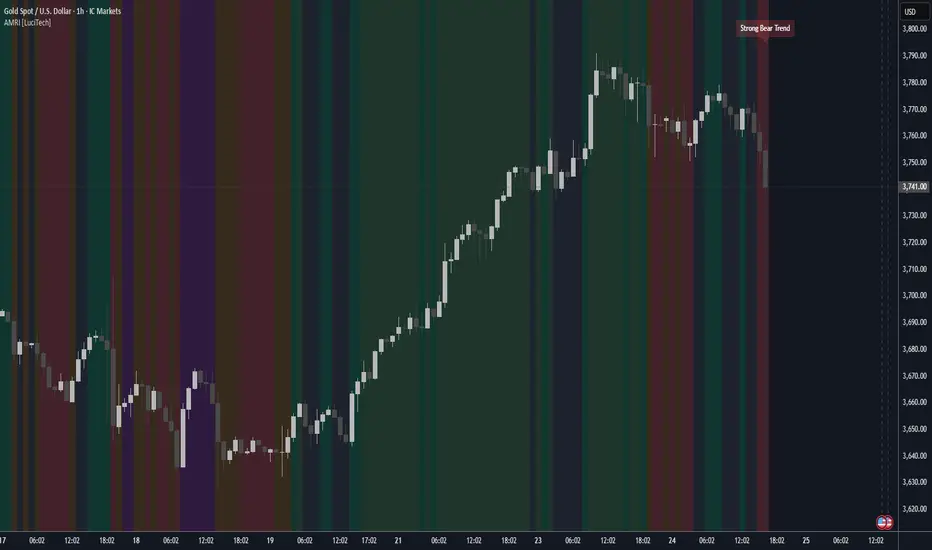
Adaptive Market Regime Identifier [LuciTech]What it Does:
AMRI visually identifies and categorizes the market into six primary regimes directly on your chart using a color-coded background. These regimes are:
-Strong Bull Trend: Characterized by robust upward momentum and low volatility.
-Weak Bull Trend: Indicates upward momentum with less conviction or higher volatility.
-Strong Bear Trend: Defined by powerful downward momentum and low volatility.
-Weak Bear Trend: Suggests downward momentum with less force or increased volatility.
-Consolidation: Periods of low volatility and sideways price action.
-Volatile Chop: High volatility without clear directional bias, often seen during transitions or indecision.
By clearly delineating these states, AMRI helps traders quickly grasp the overarching market context, enabling them to apply strategies best suited for the current conditions (e.g., trend-following in strong trends, range-bound strategies in consolidation, or caution in volatile chop).
How it Works (The Adaptive Edge)
AMRI achieves its adaptive classification by continuously analyzing three core market dimensions, with each component dynamically adjusting to current market conditions:
1.Adaptive Moving Average (KAMA): The indicator utilizes the Kaufman Adaptive Moving Average (KAMA) to gauge trend direction and strength. KAMA is unique because it adjusts its smoothing period based on market efficiency (noise vs. direction). In trending markets, it becomes more responsive, while in choppy markets, it smooths out noise, providing a more reliable trend signal than static moving averages.
2.Adaptive Average True Range (ATR): Volatility is measured using an adaptive version of the Average True Range. Similar to KAMA, this ATR dynamically adjusts its sensitivity to reflect real-time changes in market volatility. This helps AMRI differentiate between calm, ranging markets and highly volatile, directional moves or chaotic periods.
3.Normalized Slope Analysis: The slope of the KAMA is normalized against the Adaptive ATR. This normalization provides a robust measure of trend strength that is relative to the current market volatility, making the thresholds for strong and weak trends more meaningful across different instruments and timeframes.
These adaptive components work in concert to provide a nuanced and responsive classification of the market regime, minimizing lag and reducing false signals often associated with fixed-parameter indicators.
Key Features & Originality:
-Dynamic Regime Classification: AMRI stands out by not just indicating trend or range, but by classifying the type of market regime, offering a higher-level analytical framework. This is a meta-indicator that provides context for all other trading tools.
-Adaptive Core Metrics: The use of KAMA and an Adaptive ATR ensures that the indicator remains relevant and responsive across diverse market conditions, automatically adjusting to changes in volatility and trend efficiency. This self-adjusting nature is a significant advantage over indicators with static lookback periods.
-Visual Clarity: The color-coded background provides an immediate, at-a-glance understanding of the current market regime, reducing cognitive load and allowing for quicker decision-making.
-Contextual Trading: By identifying the prevailing regime, AMRI empowers traders to select and apply strategies that are most effective for that specific environment, helping to avoid costly mistakes of using a trend-following strategy in a ranging market, or vice-versa.
-Originality: While components like KAMA and ATR are known, their adaptive integration into a comprehensive, multi-regime classification system, combined with normalized slope analysis for trend strength, offers a novel approach to market analysis not commonly found in publicly available indicators.
FNGAdataCloseClose prices for FNGA ETF (Dec 2018–May 2025)
The Close prices for FNGA ETF (December 2018 – May 2025) represent the final trading price recorded at the end of each regular U.S. market session (4:00 p.m. Eastern Time) over the entire lifespan of this leveraged exchange-traded note. Initially issued under the ticker FNGU and later rebranded as FNGA in March 2025 before its redemption in May 2025, the product was designed to provide 3x daily leveraged exposure to the MicroSectors FANG+™ Index, which tracks a concentrated group of large-cap technology and tech-enabled growth leaders such as Apple, Amazon, Meta (Facebook), Netflix, and Alphabet (Google).
Close prices are widely regarded as the most important reference point in market data because they establish the official end-of-day valuation of a security. For leveraged products like FNGA, the closing price is especially critical, since it directly determines the reset value for the following trading session. This daily compounding effect means that FNGA’s closing levels often diverged significantly from the long-term performance of its underlying index, creating both opportunities and risks for traders.

FNGAdataLow“Low prices for FNGA ETF (Dec 2018–May 2025)
The Low prices for FNGA ETF (December 2018 – May 2025) capture the lowest trading price reached during each regular U.S. market session over the entire lifespan of this leveraged exchange-traded note. Initially launched under the ticker FNGU, and later rebranded as FNGA in March 2025 before its eventual redemption, the fund was structured to deliver 3x daily leveraged exposure to the MicroSectors FANG+™ Index. This index concentrated on a small basket of leading technology and tech-enabled growth companies such as Meta (Facebook), Amazon, Apple, Netflix, and Alphabet (Google), along with a few other innovators.
The Low price is particularly important in the study of FNGA because it highlights the intraday downside extremes of a highly volatile, leveraged product. Since FNGA was designed to reset leverage daily, its lows often reflected moments of amplified market stress, when declines in the underlying FANG+™ stocks were multiplied through the 3x leverage structure.

FNGAdataHighHigh prices for FNGA ETF (Dec 2018–May 2025)
The High prices for FNGA ETF (December 2018 – May 2025) represent the maximum trading price reached during each regular U.S. market session over the entire trading lifespan of this leveraged exchange-traded note. Originally issued under the ticker FNGU, and later rebranded as FNGA in March 2025 before its redemption, the fund was designed to deliver 3x daily leveraged exposure to the MicroSectors FANG+™ Index. This index focused on a concentrated group of large-cap technology and technology-enabled companies such as Facebook (Meta), Amazon, Apple, Netflix, and Google (Alphabet), along with a few other growth leaders.
The High price data from December 2018 through May 2025 is crucial for understanding how FNGA behaved during intraday trading sessions. Because FNGA was a daily resetting 3x leveraged product, its intraday highs often displayed extreme sensitivity to movements in the underlying FANG+™ stocks, resulting in sharp upward spikes during bullish days and pronounced volatility during broader market rallies.

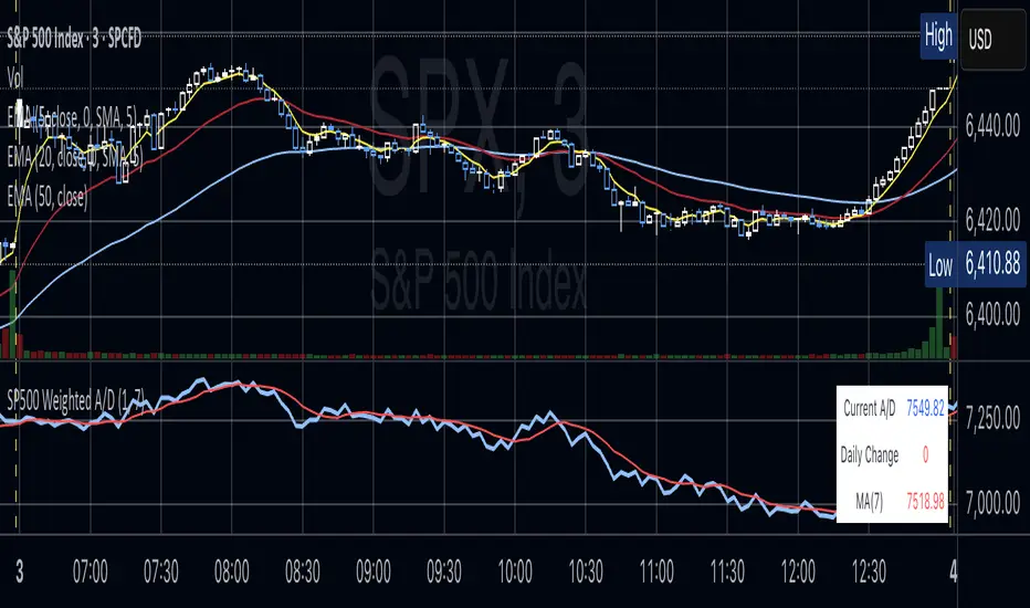
S&P 500 Weighted Advance Decline LineS&P 500 Weighted Advance Decline Line Indicator
Overview
This indicator creates a market cap weighted advance/decline line for the S&P 500 that tracks breadth based on actual index weights rather than treating all stocks equally. By weighting each stock's contribution according to its true S&P 500 impact, it provides more accurate market breadth analysis and better insights into underlying market strength and potential turning points.
Key Features
Market Cap Weighted: Each stock contributes based on its actual S&P 500 weight
Top 40 Stocks: Covers ~51% of the index with the largest companies
(limited by TradingView's 40 security call maximum for Premium accounts)
Real-Time Updates: Cumulative line shows long-term breadth trends
Visual Indicators: Background coloring, moving average option, and data table
Stock Coverage
Sector Breakdown:
Technology (29.8%) - Dominates the coverage as expected
Financials (5.8%) - Major banking and payment companies
Consumer/Retail (3.7%) - Consumer staples and retail giants
Healthcare (3.2%) - Pharma and healthcare services
Communication (1.97%) - Telecom and tech services
Energy (1.35%) - Oil and gas majors
Industrial (0.9%) - Aerospace and industrial equipment
Other Sectors (4.6%) - Miscellaneous including software and payments
Includes the 40 largest S&P 500 companies by weight, featuring:
Tech Leaders (29.8%): AAPL (7.0%), MSFT (6.5%), NVDA (4.5%), AMZN (3.5%), META (2.5%), GOOGL/GOOG (3.8%), AVGO (1.5%), ORCL (1.22%), AMD (0.51%), plus others
Financials (5.8%): BRK.B (1.8%), JPM (1.2%), V (1.0%), MA (0.8%), BAC (0.63%), WFC (0.46%)
Healthcare (3.2%): LLY (1.2%), UNH (1.2%), JNJ (1.1%), ABBV (0.8%), PG (0.9%)
Consumer/Retail (3.7%): WMT (0.8%), HD (0.8%), COST (0.7%), KO (0.6%), PEP (0.6%), NKE (0.4%)
Communication (1.97%): TMUS (0.47%), CSCO (0.47%), DIS (0.5%), CRM (0.5%)
Energy** (1.35%): XOM (0.8%), CVX (0.55%)
Industrial** (0.9%): GE (0.5%), BA (0.4%)
Other Sectors (4.6%): PLTR (0.65%), ADBE (0.6%), PYPL (0.3%), plus others
How to Interpret
Trend Signals
Rising A/D Line: Broad market strength, more weighted buying than selling
Falling A/D Line: Market weakness, more weighted selling pressure
Flat A/D Line: Balanced market conditions
Divergence Analysis
Bullish Divergence: S&P 500 makes new lows but A/D Line holds higher
Bearish Divergence: S&P 500 makes new highs but A/D Line fails to confirm
Confirmation
Strong trends occur when both price and A/D Line move in the same direction
Weak trends show when price moves but breadth doesn't follow
Settings
Lookback Period: Days for advance/decline comparison (default: 1)
Show Moving Average: Optional trend smoothing
MA Length: Moving average period (default: 20)
Limitations
Covers ~51% of S&P 500 (not complete market breadth)
Optimized for TradingView Premium accounts (40 security limit)
Heavy weighting toward mega-cap technology stocks
Dependent on real-time data quality
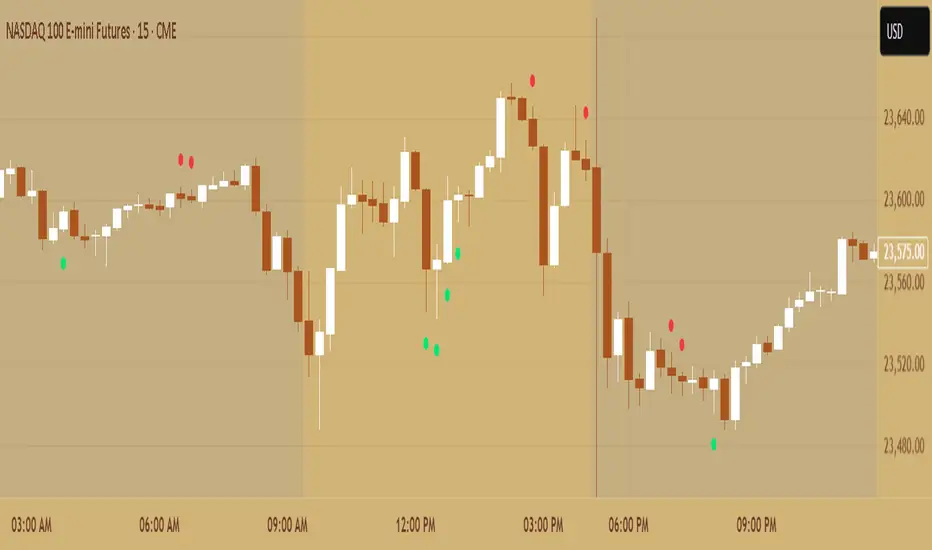
Primitive Delta DivergencePrimitive Delta Divergence
This indicator detects volume-price divergences by analyzing the relationship between price direction and volume bias over a rolling lookback period, revealing potential momentum shifts before they become apparent in price action alone.
Instead of relying solely on price movements, you can identify moments when volume sentiment contradicts price direction — a core concept borrowed from footprint chart analysis, adapted for traditional bar charts.
For example, when price moves higher but volume is predominantly bearish, or when price declines while volume shows bullish accumulation.
🔹 How it works
Lookback Period (n) → defines the rolling window for analyzing price and volume relationships
Creates a "meta-candle" from the lookback period, comparing its open vs. close for price bias
Volume classification → separates each bar's volume into bullish (green candles), bearish (red candles), or neutral (doji candles)
Volume bias calculation → generates a continuous score (-1 to +1) representing the directional volume pressure
Plots divergence signals when price direction and volume bias disagree
🔹 Use cases
Spot early momentum exhaustion when price and volume move in opposite directions
Identify potential reversal zones where volume suggests underlying weakness or strength
Enhance entry/exit timing by incorporating volume-based confirmation alongside price action
Apply footprint-style analysis to any timeframe without specialized charting tools
✨ Primitive Delta Divergence reveals the hidden story volume tells about price, uncovering divergences that traditional indicators might miss.
NAS100 Component Sentiment Scanner# NAS100 Component Sentiment Scanner
## 🎯 Overview
The NAS100 Component Sentiment Scanner analyzes the top-weighted stocks in the NASDAQ-100 index to provide real-time bullish/bearish sentiment signals that can help predict NAS100 price movements. This indicator combines multiple technical analysis methods to give traders a comprehensive view of underlying market sentiment.
## 📊 How It Works
The indicator calculates sentiment scores for major NASDAQ-100 components (AAPL, MSFT, NVDA, GOOGL, AMZN, META, TSLA, AVGO, COST, NFLX) using:
- **RSI Analysis**: Identifies overbought/oversold conditions
- **Moving Average Trends**: Compares fast vs slow MA positioning
- **Volume Confirmation**: Validates moves with volume thresholds
- **Price Momentum**: Analyzes recent price direction
- **Market Cap Weighting**: Uses actual NASDAQ-100 weightings for accuracy
## 🚀 Key Features
### Real-Time Sentiment Analysis
- Weighted composite score based on individual stock analysis
- Color-coded sentiment line (Green = Bullish, Red = Bearish)
- Dynamic background coloring for strong signals
### Interactive Data Table
- Shows individual stock scores and signals
- Bullish/Bearish stock count summary
- Customizable position and size
### Smart Signal System
- **Bullish Signals**: Green triangle up when sentiment crosses threshold
- **Bearish Signals**: Red triangle down when sentiment falls below threshold
- **Alert Conditions**: Automatic notifications for signal changes
## ⚙️ Customization Options
### Technical Analysis Settings
- **RSI Period**: Adjust lookback period (default: 14)
- **RSI Levels**: Set overbought/oversold thresholds
- **Moving Averages**: Configure fast/slow MA periods
- **Volume Threshold**: Set volume confirmation multiplier
### Signal Thresholds
- **Bullish/Bearish Levels**: Customize trigger points
- **Strong Signal Levels**: Set extreme sentiment thresholds
- Fine-tune sensitivity to market conditions
### Display Options
- **Toggle Table**: Show/hide sentiment data table
- **Table Position**: 6 position options (Top/Bottom/Middle + Left/Right)
- **Table Size**: Choose from Tiny, Small, Normal, or Large
- **Background Colors**: Enable/disable signal backgrounds
- **Signal Arrows**: Show/hide buy/sell indicators
### Stock Selection
- **Individual Control**: Enable/disable any of the 10 major stocks
- **Dynamic Weighting**: Automatically adjusts calculations based on selected stocks
- **Flexible Analysis**: Focus on specific sectors or market leaders
## 📈 How to Use
### 1. Basic Setup
1. Add the indicator to your NAS100 chart
2. Default settings work well for most traders
3. Observe the sentiment line and signals
### 2. Signal Interpretation
- **Score > 30**: Bullish bias for NAS100
- **Score > 50**: Strong bullish signal
- **Score -30 to 30**: Neutral/consolidation
- **Score < -30**: Bearish bias for NAS100
- **Score < -50**: Strong bearish signal
### 3. Trading Strategies
**Trend Following:**
- Buy NAS100 when bullish signals appear
- Sell/short when bearish signals trigger
- Use background colors for quick visual confirmation
**Divergence Trading:**
- Watch for sentiment/price divergences
- Strong sentiment with weak NAS100 price = potential breakout
- Weak sentiment with strong NAS100 price = potential reversal
**Consensus Trading:**
- Monitor bullish/bearish stock counts in table
- 8+ stocks aligned = strong directional bias
- Mixed signals = wait for clearer consensus
### 4. Advanced Usage
- Combine with your existing NAS100 trading strategy
- Use multiple timeframes for confirmation
- Adjust thresholds based on market volatility
- Focus on specific stocks by disabling others
## 🔔 Alert Setup
The indicator includes built-in alert conditions:
1. Go to TradingView Alerts
2. Select "NAS100 Component Sentiment Scanner"
3. Choose from available alert types:
- NAS100 Bullish Signal
- NAS100 Bearish Signal
- Strong Bullish Consensus
- Strong Bearish Consensus
## 💡 Pro Tips
### Optimization
- **High Volatility**: Increase signal thresholds (±40, ±60)
- **Low Volatility**: Decrease thresholds (±20, ±40)
- **Day Trading**: Use smaller table, focus on real-time signals
- **Swing Trading**: Enable background colors, larger thresholds
### Best Practices
- Don't use as a standalone system - combine with price action
- Check individual stock table for context
- Monitor during market open for most reliable signals
- Consider earnings seasons for individual stock impacts
### Market Conditions
- **Trending Markets**: Higher accuracy, use with trend following
- **Ranging Markets**: Watch for false signals, increase thresholds
- **News Events**: Individual stock news can skew sentiment temporarily
## 🎨 Visual Guide
- **Green Line Above Zero**: Bullish sentiment building
- **Red Line Below Zero**: Bearish sentiment building
- **Background Color Changes**: Strong signal confirmation
- **Triangle Arrows**: Entry/exit signal points
- **Table Colors**: Quick sentiment overview
## ⚠️ Important Notes
- This indicator analyzes component stocks, not NAS100 directly
- Market cap weightings approximate real NASDAQ-100 weightings
- Sentiment can change rapidly during volatile periods
- Always use proper risk management
- Combine with other technical analysis tools
## 🔧 Troubleshooting
- **No signals**: Check if thresholds are too extreme
- **Too many signals**: Increase threshold sensitivity
- **Table not showing**: Ensure "Show Sentiment Table" is enabled
- **Missing stocks**: Verify individual stock toggles in settings
---
**Suitable for**: Day traders, swing traders, NAS100 specialists, index traders
**Best Timeframes**: 5min, 15min, 1H, 4H
**Market Sessions**: US market hours for highest accuracy

Correlation HeatMap Matrix Data [TradingFinder]🔵 Introduction
Correlation is a statistical measure that shows the degree and direction of a linear relationship between two assets.
Its value ranges from -1 to +1 : +1 means perfect positive correlation, 0 means no linear relationship, and -1 means perfect negative correlation.
In financial markets, correlation is used for portfolio diversification, risk management, pairs trading, intermarket analysis, and identifying divergences.
Correlation HeatMap Matrix Data TradingFinder is a Pine Script v6 library that calculates and returns raw correlation matrix data between up to 20 symbols. It only provides the data – it does not draw or render the heatmap – making it ideal for use in other scripts that handle visualization or further analysis. The library uses ta.correlation for fast and accurate calculations.
It also includes two helper functions for visual styling :
CorrelationColor(corr) : takes the correlation value as input and generates a smooth gradient color, ranging from strong negative to strong positive correlation.
CorrelationTextColor(corr) : takes the correlation value as input and returns a text color that ensures optimal contrast over the background color.
Library
"Correlation_HeatMap_Matrix_Data_TradingFinder"
CorrelationColor(corr)
Parameters:
corr (float)
CorrelationTextColor(corr)
Parameters:
corr (float)
Data_Matrix(Corr_Period, Sym_1, Sym_2, Sym_3, Sym_4, Sym_5, Sym_6, Sym_7, Sym_8, Sym_9, Sym_10, Sym_11, Sym_12, Sym_13, Sym_14, Sym_15, Sym_16, Sym_17, Sym_18, Sym_19, Sym_20)
Parameters:
Corr_Period (int)
Sym_1 (string)
Sym_2 (string)
Sym_3 (string)
Sym_4 (string)
Sym_5 (string)
Sym_6 (string)
Sym_7 (string)
Sym_8 (string)
Sym_9 (string)
Sym_10 (string)
Sym_11 (string)
Sym_12 (string)
Sym_13 (string)
Sym_14 (string)
Sym_15 (string)
Sym_16 (string)
Sym_17 (string)
Sym_18 (string)
Sym_19 (string)
Sym_20 (string)
🔵 How to use
Import the library into your Pine Script using the import keyword and its full namespace.
Decide how many symbols you want to include in your correlation matrix (up to 20). Each symbol must be provided as a string, for example FX:EURUSD .
Choose the correlation period (Corr\_Period) in bars. This is the lookback window used for the calculation, such as 20, 50, or 100 bars.
Call Data_Matrix(Corr_Period, Sym_1, ..., Sym_20) with your selected parameters. The function will return an array containing the correlation values for every symbol pair (upper triangle of the matrix plus diagonal).
For example :
var string Sym_1 = '' , var string Sym_2 = '' , var string Sym_3 = '' , var string Sym_4 = '' , var string Sym_5 = '' , var string Sym_6 = '' , var string Sym_7 = '' , var string Sym_8 = '' , var string Sym_9 = '' , var string Sym_10 = ''
var string Sym_11 = '', var string Sym_12 = '', var string Sym_13 = '', var string Sym_14 = '', var string Sym_15 = '', var string Sym_16 = '', var string Sym_17 = '', var string Sym_18 = '', var string Sym_19 = '', var string Sym_20 = ''
switch Market
'Forex' => Sym_1 := 'EURUSD' , Sym_2 := 'GBPUSD' , Sym_3 := 'USDJPY' , Sym_4 := 'USDCHF' , Sym_5 := 'USDCAD' , Sym_6 := 'AUDUSD' , Sym_7 := 'NZDUSD' , Sym_8 := 'EURJPY' , Sym_9 := 'EURGBP' , Sym_10 := 'GBPJPY'
,Sym_11 := 'AUDJPY', Sym_12 := 'EURCHF', Sym_13 := 'EURCAD', Sym_14 := 'GBPCAD', Sym_15 := 'CADJPY', Sym_16 := 'CHFJPY', Sym_17 := 'NZDJPY', Sym_18 := 'AUDNZD', Sym_19 := 'USDSEK' , Sym_20 := 'USDNOK'
'Stock' => Sym_1 := 'NVDA' , Sym_2 := 'AAPL' , Sym_3 := 'GOOGL' , Sym_4 := 'GOOG' , Sym_5 := 'META' , Sym_6 := 'MSFT' , Sym_7 := 'AMZN' , Sym_8 := 'AVGO' , Sym_9 := 'TSLA' , Sym_10 := 'BRK.B'
,Sym_11 := 'UNH' , Sym_12 := 'V' , Sym_13 := 'JPM' , Sym_14 := 'WMT' , Sym_15 := 'LLY' , Sym_16 := 'ORCL', Sym_17 := 'HD' , Sym_18 := 'JNJ' , Sym_19 := 'MA' , Sym_20 := 'COST'
'Crypto' => Sym_1 := 'BTCUSD' , Sym_2 := 'ETHUSD' , Sym_3 := 'BNBUSD' , Sym_4 := 'XRPUSD' , Sym_5 := 'SOLUSD' , Sym_6 := 'ADAUSD' , Sym_7 := 'DOGEUSD' , Sym_8 := 'AVAXUSD' , Sym_9 := 'DOTUSD' , Sym_10 := 'TRXUSD'
,Sym_11 := 'LTCUSD' , Sym_12 := 'LINKUSD', Sym_13 := 'UNIUSD', Sym_14 := 'ATOMUSD', Sym_15 := 'ICPUSD', Sym_16 := 'ARBUSD', Sym_17 := 'APTUSD', Sym_18 := 'FILUSD', Sym_19 := 'OPUSD' , Sym_20 := 'USDT.D'
'Custom' => Sym_1 := Sym_1_C , Sym_2 := Sym_2_C , Sym_3 := Sym_3_C , Sym_4 := Sym_4_C , Sym_5 := Sym_5_C , Sym_6 := Sym_6_C , Sym_7 := Sym_7_C , Sym_8 := Sym_8_C , Sym_9 := Sym_9_C , Sym_10 := Sym_10_C
,Sym_11 := Sym_11_C, Sym_12 := Sym_12_C, Sym_13 := Sym_13_C, Sym_14 := Sym_14_C, Sym_15 := Sym_15_C, Sym_16 := Sym_16_C, Sym_17 := Sym_17_C, Sym_18 := Sym_18_C, Sym_19 := Sym_19_C , Sym_20 := Sym_20_C
= Corr.Data_Matrix(Corr_period, Sym_1 ,Sym_2 ,Sym_3 ,Sym_4 ,Sym_5 ,Sym_6 ,Sym_7 ,Sym_8 ,Sym_9 ,Sym_10,Sym_11,Sym_12,Sym_13,Sym_14,Sym_15,Sym_16,Sym_17,Sym_18,Sym_19,Sym_20)
Loop through or index into this array to retrieve each correlation value for your custom layout or logic.
Pass each correlation value to CorrelationColor() to get the corresponding gradient background color, which reflects the correlation’s strength and direction (negative to positive).
For example :
Corr.CorrelationColor(SYM_3_10)
Pass the same correlation value to CorrelationTextColor() to get the correct text color for readability against that background.
For example :
Corr.CorrelationTextColor(SYM_1_1)
Use these colors in a table or label to render your own heatmap or any other visualization you need.

Dark Pool Block Trades - Institutional Volume📊 Dark Pool Block Trades - Institutional Volume
Visualize where institutional money positions before major price moves occur. This indicator reveals hidden dark pool block trades that often precede significant price movements - because when smart money deploys millions and billions in strategic accumulation or distribution, retail traders need to see where it's happening.
🎯 WHY DARK POOL DATA MATTERS:
Institutions don't move large capital randomly. Dark pool block trades represent strategic positioning by sophisticated money managers with superior research and conviction. These trades create hidden support/resistance levels that often predict future price action.
The key principle: Follow institutional flow, don't fight it. When institutions get involved, they create high-probability trading opportunities.
💰 HOW INSTITUTIONS INFLUENCE PRICE:
- Large block trades establish hidden accumulation/distribution zones
- Smart money builds positions BEFORE retail awareness increases
- Institutional activity creates "footprints" at key technical levels
- These trades often signal conviction plays ahead of major moves
- Institutions typically add to winning positions throughout trends
🔍 WHAT THIS INDICATOR SHOWS:
- Visual overlay of dark pool block trades directly on price charts
- Track institutional positioning across major stocks and ETFs
- Identify accumulation/distribution zones before they become obvious to retail
- Spot high-conviction institutional trades in real-time visualization
- Customizable block trade size filters and timeframe selection
- Historical institutional activity up to 5 years or custom ranges
💡 THE TRADING ADVANTAGE:
Instead of guessing price direction, see where institutions are already positioning. When large block trades appear in dark pools, you're witnessing strategic institutional commitment that frequently leads to significant price movements.
⚡ HOW IT WORKS:
This Pine Script displays institutional dark pool transactions as visual markers on your charts. The script comes with sample data for immediate use. For expanded ticker coverage and real-time updates, external data services are available.
🎯 IDEAL FOR:
- Swing traders following institutional footprints
- Traders seeking setups backed by smart money conviction
- Position traders looking for accumulation zones
- Anyone wanting to align with institutional flow rather than fight it
🔄 SAMPLE DATA INCLUDED:
Pre-loaded with institutional activity data across popular tickers, updated daily to demonstrate how dark pool activity correlates with future price movements.
The script initially covers these tickers going back 6 months showing the top 10 trades by volume over 400,000 shares: AAPL, AMD, AMZN, ARKK, ARKW, BAC, BITO, COIN, COST, DIA, ETHA, GLD, GOOGL, HD, HYG, IBB, IWM, JNJ, JPM, LQD, MA, META, MSFT, NVDA, PG, QQQ, RIOT, SLV, SMCI, SMH, SOXX, SPY, TLT, TSLA, UNH, USO, V, VEA, VNQ, VOO, VTI, VWO, WMT, XLE, XLF, XLK, XLU, XLV, XLY

SIC_TICKER_DATAThe SIC Ticker Data is an advanced and efficient library for ticker-to-industry classification and sector analysis. Built with enterprise-grade performance optimizations, this library provides instant access to SIC codes, industry classifications, and peer company data for comprehensive market analysis.
Perfect for: Sector rotation strategies, peer analysis, portfolio diversification, market screening, and financial research tools.
The simple idea behind this library is to pull any data related to SIC number of any US stock market ticker provided by SEC in order to see the industry and also see the exact competitors of the ticker.
The library stores 3 types of data: SIC number, Ticker, and Industry name. What makes it very useful is that you can pull any one of this data using the other. For example, if you would like to know which tickers are inside a certain SIC, or what's the SIC number of a specific ticker, or even which tickers are inside a certain industry, you can use this library to pull this data. The idea for data inside this library is to be accessible in any direction possible as long as they're related to each other.
We've also published a simple indicator that uses this library in order to demonstrate the inner workings of this library.
The library stores thousands of tickers and their relevant SIC code and industry for your use and is constantly updated with new data when available. This is a large library but it is optimized to run as fast as possible. The previous unpublished versions would take over 40 seconds to load any data but the final public version here loads the data in less than 5 seconds.
🔍 Primary Lookup Functions
createDataStore()
Initialize the library with all pre-loaded data.
store = data.createDataStore()
getSicByTicker(store, ticker)
Get SIC code for any ticker symbol.
sic = data.getSicByTicker(store, "AAPL") // Returns: "3571"
getIndustryByTicker(store, ticker)
Get industry classification for any ticker.
industry = data.getIndustryByTicker(store, "AAPL") // Returns: "Computer Hardware"
getTickersBySic(store, sic)
Get all companies in a specific SIC code.
software = data.getTickersBySic(store, "7372") // Returns: "MSFT,GOOGL,META,V,MA,CRM,ADBE,ORCL,NOW,INTU"
getTickersByIndustry(store, industry)
Get all companies in an industry.
retail = data.getTickersByIndustry(store, "Retail") // Returns: "AMZN,HD,WMT,TGT,COST,LOW"
📊 Array & Analysis Functions
getTickerArrayBySic(store, sic)
Get tickers as array for processing.
techArray = data.getTickerArrayBySic(store, "7372")
for i = 0 to array.size(techArray) - 1
ticker = array.get(techArray, i)
// Process each tech company
getTickerCountBySic(store, sic)
Count companies in a sector (ultra-fast).
pinescripttechCount = data.getTickerCountBySic(store, "7372") // Returns: 10
🎯 Utility Functions
tickerExists(store, ticker)
Check if ticker exists in database.
exists = data.tickerExists(store, "AAPL") // Returns: true
tickerInSic(store, ticker, sic)
Check if ticker belongs to specific sector.
isInTech = data.tickerInSic(store, "AAPL", "3571") // Returns: true
💡 Usage Examples
Example 1: Basic Ticker Lookup
// @version=6
import EdgeTerminal/SIC_TICKER_DATA/1 as data
indicator("Ticker Analysis", overlay=true)
store = data.createDataStore()
currentSic = data.getSicByTicker(store, syminfo.ticker)
currentIndustry = data.getIndustryByTicker(store, syminfo.ticker)
if barstate.islast and currentSic != "NOT_FOUND"
label.new(bar_index, high, syminfo.ticker + "\nSIC: " + currentSic + "\nIndustry: " + currentIndustry)
Example 2: Sector Analysis
// @version=6
import EdgeTerminal/SIC_TICKER_DATA/1 as data
indicator("Sector Comparison", overlay=false)
store = data.createDataStore()
// Compare sector sizes
techCount = data.getTickerCountBySic(store, "7372") // Software
financeCount = data.getTickerCountBySic(store, "6199") // Finance
healthCount = data.getTickerCountBySic(store, "2834") // Pharmaceutical
plot(techCount, title="Tech Companies", color=color.blue)
plot(financeCount, title="Finance Companies", color=color.green)
plot(healthCount, title="Health Companies", color=color.red)
Example 3: Peer Analysis
// @version=6
import EdgeTerminal/SIC_TICKER_DATA/1 as data
indicator("Find Competitors", overlay=true)
store = data.createDataStore()
currentSic = data.getSicByTicker(store, syminfo.ticker)
if currentSic != "NOT_FOUND"
competitors = data.getTickersBySic(store, currentSic)
peerCount = data.getTickerCountBySic(store, currentSic)
if barstate.islast
label.new(bar_index, high, "Competitors (" + str.tostring(peerCount) + "):\n" + competitors)
Example 4: Portfolio Sector Allocation
// @version=6
import EdgeTerminal/SIC_TICKER_DATA/1 as data
indicator("Portfolio Analysis", overlay=false)
store = data.createDataStore()
// Analyze your portfolio's sector distribution
portfolioTickers = array.from("AAPL", "MSFT", "GOOGL", "JPM", "JNJ")
sectorCount = map.new()
for i = 0 to array.size(portfolioTickers) - 1
ticker = array.get(portfolioTickers, i)
industry = data.getIndustryByTicker(store, ticker)
if industry != "NOT_FOUND"
currentCount = map.get(sectorCount, industry)
newCount = na(currentCount) ? 1 : currentCount + 1
map.put(sectorCount, industry, newCount)
🔧 Advanced Feature
You can also bulk load data for large data sets like this:
// Pre-format your data as pipe-separated string
bulkData = "AAPL:3571:Computer Hardware|MSFT:7372:Software|GOOGL:7372:Software"
store = data.createDataStoreFromBulk(bulkData)
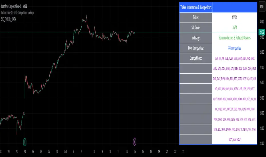
Options Strategy V1.3📈 Options Strategy V1.3 — EMA Crossover + RSI + ATR + Opening Range
Overview:
This strategy is designed for short-term directional trades on large-cap stocks or ETFs, especially when trading options. It combines classic trend-following signals with momentum confirmation, volatility-based risk management, and session timing filters to help identify high-probability entries with predefined stop-loss and profit targets.
🔍 Strategy Components:
EMA Crossover (Fast/Slow)
Entry signals are triggered by the crossover of a short EMA above or below a long EMA — a traditional trend-following method to detect shifts in momentum.
RSI Filter
RSI confirms the signal by avoiding entries in overbought/oversold zones unless certain momentum conditions are met.
Long entry requires RSI ≥ Long Threshold
Short entry requires RSI ≤ Short Threshold
ATR-Based SL & TP
Stop-loss is set dynamically as a multiple of ATR below (long) or above (short) the entry price.
Take-profit is placed as a ratio (TP/SL) of the stop distance, ensuring consistent reward/risk structure.
Opening Range Filter (Optional)
If enabled, the strategy only triggers trades after price breaks out of the 09:30–09:45 EST range, ensuring participation in directional moves.
Session Filters
No trades from 04:00 to 09:30 and from 16:00 to 20:00 EST, avoiding low-liquidity periods.
All open trades are closed at 15:55 EST, to avoid overnight risk or expiration issues for options.
⚙️ Built-in Presets:
You can choose one of the built-in ticker-specific presets for optimal conditions:
Ticker EMAs RSI (Long/Short) ATR SL×ATR TP/SL
SPY 8/28 56 / 26 14 1.4× 4.0×
TSLA 23/27 56 / 33 13 1.4× 3.6×
AAPL 6/13 61 / 26 23 1.4× 2.1×
MSFT 25/32 54 / 26 14 1.2× 2.2×
META 25/32 53 / 26 17 1.8× 2.3×
AMZN 28/32 55 / 25 16 1.8× 2.3×
You can also choose "Custom" to fully configure all parameters to your own market and strategy preferences.
📌 Best Use Case:
This strategy is especially suited for intraday options trading, where timing and risk control are critical. It works best on liquid tickers with strong trends or clear breakout behavior.

Magnificent 7 OscillatorThe Magnificent 7 Oscillator is a sophisticated momentum-based technical indicator designed to analyze the collective performance of the seven largest technology companies in the U.S. stock market (Apple, Microsoft, Alphabet, Amazon, NVIDIA, Tesla, and Meta). This indicator incorporates established momentum factor research and provides three distinct analytical modes: absolute momentum tracking, equal-weighted market comparison, and relative performance analysis. The tool integrates five different oscillator methodologies and includes advanced breadth analysis capabilities.
Theoretical Foundation
Momentum Factor Research
The indicator's foundation rests on seminal momentum research in financial markets. Jegadeesh and Titman (1993) demonstrated that stocks with strong price performance over 3-12 month periods tend to continue outperforming in subsequent periods¹. This momentum effect was later incorporated into formal factor models by Carhart (1997), who extended the Fama-French three-factor model to include a momentum factor (UMD - Up Minus Down)².
The momentum calculation methodology follows the academic standard:
Momentum(t) = / P(t-n) × 100
Where P(t) is the current price and n is the lookback period.
The focus on the "Magnificent 7" stocks reflects the increasing market concentration observed in recent years. Fama and French (2015) noted that a small number of large-cap stocks can drive significant market movements due to their substantial index weights³. The combined market capitalization of these seven companies often exceeds 25% of the total S&P 500, making their collective momentum a critical market indicator.
Indicator Architecture
Core Components
1. Data Collection and Processing
The indicator employs robust data collection with error handling for missing or invalid security data. Each stock's momentum is calculated independently using the specified lookback period (default: 14 periods).
2. Composite Oscillator Calculation
Following Fama-French factor construction methodology, the indicator offers two weighting schemes:
- Equal Weight: Each active stock receives identical weighting (1/n)
- Market Cap Weight: Reserved for future enhancement
3. Oscillator Transformation Functions
The indicator provides five distinct oscillator types, each with established technical analysis foundations:
a) Momentum Oscillator (Default)
- Pure rate-of-change calculation
- Centered around zero
- Direct implementation of Jegadeesh & Titman methodology
b) RSI (Relative Strength Index)
- Wilder's (1978) relative strength methodology
- Transformed to center around zero for consistency
- Scale: -50 to +50
c) Stochastic Oscillator
- George Lane's %K methodology
- Measures current position within recent range
- Transformed to center around zero
d) Williams %R
- Larry Williams' range-based oscillator
- Inverse stochastic calculation
- Adjusted for zero-centered display
e) CCI (Commodity Channel Index)
- Donald Lambert's mean reversion indicator
- Measures deviation from moving average
- Scaled for optimal visualization
Operational Modes
Mode 1: Magnificent 7 Analysis
Tracks the collective momentum of the seven constituent stocks. This mode is optimal for:
- Technology sector analysis
- Growth stock momentum assessment
- Large-cap performance tracking
Mode 2: S&P 500 Equal Weight Comparison
Analyzes momentum using an equal-weighted S&P 500 reference (typically RSP ETF). This mode provides:
- Broader market momentum context
- Size-neutral market analysis
- Comparison baseline for relative performance
Mode 3: Relative Performance Analysis
Calculates the momentum differential between Magnificent 7 and S&P 500 Equal Weight. This mode enables:
- Sector rotation analysis
- Style factor assessment (Growth vs. Value)
- Relative strength identification
Formula: Relative Performance = MAG7_Momentum - SP500EW_Momentum
Signal Generation and Thresholds
Signal Classification
The indicator generates three signal states:
- Bullish: Oscillator > Upper Threshold (default: +2.0%)
- Bearish: Oscillator < Lower Threshold (default: -2.0%)
- Neutral: Oscillator between thresholds
Relative Performance Signals
In relative performance mode, specialized thresholds apply:
- Outperformance: Relative momentum > +1.0%
- Underperformance: Relative momentum < -1.0%
Alert System
Comprehensive alert conditions include:
- Threshold crossovers (bullish/bearish signals)
- Zero-line crosses (momentum direction changes)
- Relative performance shifts
- Breadth Analysis Component
The indicator incorporates market breadth analysis, calculating the percentage of constituent stocks with positive momentum. This feature provides insights into:
- Strong Breadth (>60%): Broad-based momentum
- Weak Breadth (<40%): Narrow momentum leadership
- Mixed Breadth (40-60%): Neutral momentum distribution
Visual Design and User Interface
Theme-Adaptive Display
The indicator automatically adjusts color schemes for dark and light chart themes, ensuring optimal visibility across different user preferences.
Professional Data Table
A comprehensive data table displays:
- Current oscillator value and percentage
- Active mode and oscillator type
- Signal status and strength
- Component breakdowns (in relative performance mode)
- Breadth percentage
- Active threshold levels
Custom Color Options
Users can override default colors with custom selections for:
- Neutral conditions (default: Material Blue)
- Bullish signals (default: Material Green)
- Bearish signals (default: Material Red)
Practical Applications
Portfolio Management
- Sector Allocation: Use relative performance mode to time technology sector exposure
- Risk Management: Monitor breadth deterioration as early warning signal
- Entry/Exit Timing: Utilize threshold crossovers for position sizing decisions
Market Analysis
- Trend Identification: Zero-line crosses indicate momentum regime changes
- Divergence Analysis: Compare MAG7 performance against broader market
- Volatility Assessment: Oscillator range and frequency provide volatility insights
Strategy Development
- Factor Timing: Implement growth factor timing strategies
- Momentum Strategies: Develop systematic momentum-based approaches
- Risk Parity: Use breadth metrics for risk-adjusted portfolio construction
Configuration Guidelines
Parameter Selection
- Momentum Period (5-100): Shorter periods (5-20) for tactical analysis, longer periods (50-100) for strategic assessment
- Smoothing Period (1-50): Higher values reduce noise but increase lag
- Thresholds: Adjust based on historical volatility and strategy requirements
Timeframe Considerations
- Daily Charts: Optimal for swing trading and medium-term analysis
- Weekly Charts: Suitable for long-term trend analysis
- Intraday Charts: Useful for short-term tactical decisions
Limitations and Considerations
Market Concentration Risk
The indicator's focus on seven stocks creates concentration risk. During periods of significant rotation away from large-cap technology stocks, the indicator may not represent broader market conditions.
Momentum Persistence
While momentum effects are well-documented, they are not permanent. Jegadeesh and Titman (1993) noted momentum reversal effects over longer time horizons (2-5 years).
Correlation Dynamics
During market stress, correlations among the constituent stocks may increase, reducing the diversification benefits and potentially amplifying signal intensity.
Performance Metrics and Backtesting
The indicator includes hidden plots for comprehensive backtesting:
- Individual stock momentum values
- Composite breadth percentage
- S&P 500 Equal Weight momentum
- Relative performance calculations
These metrics enable quantitative strategy development and historical performance analysis.
References
¹Jegadeesh, N., & Titman, S. (1993). Returns to buying winners and selling losers: Implications for stock market efficiency. Journal of Finance, 48(1), 65-91.
Carhart, M. M. (1997). On persistence in mutual fund performance. Journal of Finance, 52(1), 57-82.
Fama, E. F., & French, K. R. (2015). A five-factor asset pricing model. Journal of Financial Economics, 116(1), 1-22.
Wilder, J. W. (1978). New concepts in technical trading systems. Trend Research.
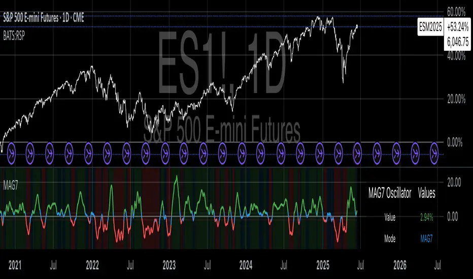
(FVC) Fractal Volatility Compression (DAFE) (FVC) Fractal Volatility Compression
See the Market’s Volatility DNA.
The Fractal Volatility Compression (FVC) is a next-generation tool for traders who want to see volatility compression and expansion across multiple timeframes and volatility engines—not just price, but the very structure of volatility itself.
What Makes FVC Unique?
Dual-Engine Volatility:
Plots both classic price-based (Stdev) and meta-volatility (VoVix) compression/expansion, so you can see when the market is “coiling” or “exploding” on multiple levels.
Fractal, Multi-Timeframe Analysis:
Measures volatility on short, medium, and long timeframes, then normalizes each as a Z-score. The result: a true “coiled spring” detector that works on any asset, any timeframe.
Threshold Lines You Control:
Yellow center line: Your neutral baseline.
Green compression line: When crossed, the market is “spring-loading.”
Red expansion line: When crossed, volatility is breaking out.
All lines are solid, clean, and end before the dashboard for a professional look.
Agreement Fill: When both engines agree (both above or both below the center line), a bright fill highlights the zone—red for expansion, green for compression.
Signature Dashboard & Info Line:
Dashboard (right-middle) shows all Z-scores and FVC values, color-coded for instant clarity.
Compact info label for mobile or minimalist users.
Inputs & Customization
Thresholds: Set the yellow, green, and red lines to match your asset, timeframe, and risk tolerance.
Timeframes & Lengths: Tune the short, medium, and long volatility windows for your style.
Toggle Lines: Show/hide Stdev or VoVix FVC lines independently.
Dashboard & Info Line: Toggle for your workflow and screen size.
How to Use
Compression (below green): Market is “coiling” across timeframes—watch for explosive moves.
Expansion (above red): Volatility is breaking out—expect regime shifts or trend acceleration.
Agreement Fill: When both lines agree, the signal is strongest.
Not a Buy/Sell Signal: These are regime and structure signals—combine with your own
strategy and risk management.
Why should you use FVC?
See what others can’t:
Most tools show only one dimension of volatility. FVC reveals the fractal DNA of market compression and expansion. Works on any asset, any timeframe. Professional, clean, and fully customizable.
Fractal Volatility Compression (FVC):
Because the next big move is born in the market’s hidden compression.
For educational purposes only. Not financial advice. Always use proper risk management
Use with discipline. Trade your edge.
— Dskyz, for DAFE Trading Systems

SuperTrader Trend Analysis and Trade Study DashboardSuperTrader Trend Analysis and Trade Study Dashboard
Overview
This script offers a multi-faceted look at market behavior. It combines signals from different momentum indicators, daily cross checks, and a specialized dashboard to reveal trend strength, potential divergences, and how far price has traveled from its recent averages.
Three Musketeers Method
This script uses a special set of three indicators (the “Three Musketeers”) to determine bullish or bearish pressure on the current chart.
Trend Condition – Compares fast vs. slow EMAs (50 and 200) and checks which side of the line price is favoring.
Mean Reversion Condition – Watches RSI crossing typical oversold or overbought thresholds (e.g., crossing above 30 or below 70).
Bollinger Condition – Checks whether price pushes above/below the Bollinger Bands (based on a 20 SMA + standard deviations).
When at least two out of these three conditions align in a bullish way, the script issues a Buy Signal . Conversely, if at least two align in a bearish way, a Sell Signal is triggered. This “Three Musketeers” synergy ensures multiple confirmations before calling a potential market turn.
Mag 8 Daily Performance
The script tracks eight highly influential stocks (AAPL, AMZN, GOOG, NFLX, NVDA, TSLA, META, MSFT) to see which are green (higher) or red (lower) compared to yesterday’s close. It then prints a quick tally – helpful in gauging overall market mood via these major players.
Golden / Death Cross Signals
On a daily time frame, the script notes when the 50-day SMA crosses above or below the 200-day SMA. A “Golden Cross” often signals rising momentum, while a “Death Cross” can hint at oncoming weakness.
RSI & Divergence Checks
RSI helps identify hidden turning points. Whenever a bullish or bearish divergence is spotted, the script updates you via a concise readout.
Hardcoded Settings
EMA lengths for trend checks, Bollinger parameters, etc., are locked in, letting you focus on adjusting only the pivotal study inputs (e.g., RSI length, VIDYA momentum).
VIDYA Trend Line & Fill
Built on an adaptive Variable Index Dynamic Average, it plots a line that quickly reacts to changing momentum. Users can set a “Trend Band Distance” to mark ATR-based thresholds around that line, identifying possible breakouts or breakdowns.
YoYo Distance
This concept measures how far price strays from SMA(10). If it’s too far, the script colors your display to indicate potential snapbacks.
Gap Up/Down Probability
By weighing volume, MACD signals, and whether price sits above/below its midrange, the script estimates probabilities of a gap up or down on the next daily candle.
Table Output & Trend Label
Turning on Show Table Widget reveals a quick dashboard on the chart detailing RSI, CCI, divergences, bull/bear scores, and more. A label on the last bar further summarizes overall trend, gap distance, and the Mag 8 snapshot – perfect for a fast read of current market posture.
Use this script to unify multiple signals in one place, see how far price has ventured from typical patterns, and get daily cross signals plus real-time bullish/bearish calls – all at a glance.
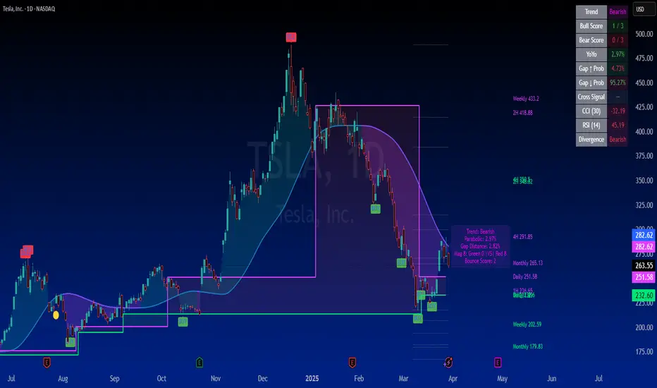
Cumulative Weighted Change (Session) with 14 MAThis indicator provides the session weighted cumulative change of the Magnificent 7(AAPL META GOOG AMZN MSFT NVDA TSLA), it is weighted according to their market capitalization and size in relation to size of the market. The bar to bar current change is plotted by the fast line that begins its calculations at the start of each daily session, the smoother(slower) line is the 14 period Volume Weighted Moving Average of the cumulative change.
I use this in conjunction with a timeframe continuity indicator in order to weed out invalid signals, I have one that I have recently published. I use this to trade futures and index stock options, since the 7 tickers that this indicator is built off of are the biggest force that moves markets this ends up acting as an alpha indicator if you can find a consistent and reliable way to weed out false signals.
Happy Trading!
-Drgzzz
