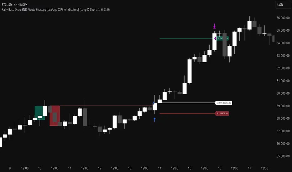
Rally Base Drop SND Pivots Strategy [LuxAlgo X PineIndicators]This strategy is based on the Rally Base Drop (RBD) SND Pivots indicator developed by LuxAlgo. Full credit for the concept and original indicator goes to LuxAlgo.
The Rally Base Drop SND Pivots Strategy is a non-repainting supply and demand trading system that detects pivot points based on Rally, Base, and Drop (RBD) candles. This strategy automatically identifies key market structure levels, allowing traders to:
Identify pivot-based supply and demand (SND) zones.
Use fixed criteria for trend continuation or reversals.
Filter out market noise by requiring structured price formations.
Enter trades based on breakouts of key SND pivot levels.
How the Rally Base Drop SND Pivots Strategy Works
1. Pivot Point Detection Using RBD Candles
The strategy follows a rigid market structure methodology, where pivots are detected only when:
A Rally (R) consists of multiple consecutive bullish candles.
A Drop (D) consists of multiple consecutive bearish candles.
A Base (B) is identified as a transition between Rallies and Drops, acting as a pivot point.
The pivot level is confirmed when the formation is complete.
Unlike traditional fractal-based pivots, RBD Pivots enforce stricter structural rules, ensuring that each pivot:
Has a well-defined bullish or bearish price movement.
Reduces false signals caused by single-bar fluctuations.
Provides clear supply and demand levels based on structured price movements.
These pivot levels are drawn on the chart using color-coded boxes:
Green zones represent bullish pivot levels (Rally Base formations).
Red zones represent bearish pivot levels (Drop Base formations).
Once a pivot is confirmed, the high or low of the base candle is used as the reference level for future trades.
2. Trade Entry Conditions
The strategy allows traders to select from three trading modes:
Long Only – Only takes long trades when bullish pivot breakouts occur.
Short Only – Only takes short trades when bearish pivot breakouts occur.
Long & Short – Trades in both directions based on pivot breakouts.
Trade entry signals are triggered when price breaks through a confirmed pivot level:
Long Entry:
A bullish pivot level is formed.
Price breaks above the bullish pivot level.
The strategy enters a long position.
Short Entry:
A bearish pivot level is formed.
Price breaks below the bearish pivot level.
The strategy enters a short position.
The strategy includes an optional mode to reverse long and short conditions, allowing traders to experiment with contrarian entries.
3. Exit Conditions Using ATR-Based Risk Management
This strategy uses the Average True Range (ATR) to calculate dynamic stop-loss and take-profit levels:
Stop-Loss (SL): Placed 1 ATR below entry for long trades and 1 ATR above entry for short trades.
Take-Profit (TP): Set using a Risk-Reward Ratio (RR) multiplier (default = 6x ATR).
When a trade is opened:
The entry price is recorded.
ATR is calculated at the time of entry to determine stop-loss and take-profit levels.
Trades exit automatically when either SL or TP is reached.
If reverse conditions mode is enabled, stop-loss and take-profit placements are flipped.
Visualization & Dynamic Support/Resistance Levels
1. Pivot Boxes for Market Structure
Each pivot is marked with a colored box:
Green boxes indicate bullish demand zones.
Red boxes indicate bearish supply zones.
These boxes remain on the chart to act as dynamic support and resistance levels, helping traders identify key price reaction zones.
2. Horizontal Entry, Stop-Loss, and Take-Profit Lines
When a trade is active, the strategy plots:
White line → Entry price.
Red line → Stop-loss level.
Green line → Take-profit level.
Labels display the exact entry, SL, and TP values, updating dynamically as price moves.
Customization Options
This strategy offers multiple adjustable settings to optimize performance for different market conditions:
Trade Mode Selection → Choose between Long Only, Short Only, or Long & Short.
Pivot Length → Defines the number of required Rally & Drop candles for a pivot.
ATR Exit Multiplier → Adjusts stop-loss distance based on ATR.
Risk-Reward Ratio (RR) → Modifies take-profit level relative to risk.
Historical Lookback → Limits how far back pivot zones are displayed.
Color Settings → Customize pivot box colors for bullish and bearish setups.
Considerations & Limitations
Pivot Breakouts Do Not Guarantee Reversals. Some pivot breaks may lead to continuation moves instead of trend reversals.
Not Optimized for Low Volatility Conditions. This strategy works best in trending markets with strong momentum.
ATR-Based Stop-Loss & Take-Profit May Require Optimization. Different assets may require different ATR multipliers and RR settings.
Market Noise May Still Influence Pivots. While this method filters some noise, fake breakouts can still occur.
Conclusion
The Rally Base Drop SND Pivots Strategy is a non-repainting supply and demand system that combines:
Pivot-based market structure analysis (using Rally, Base, and Drop candles).
Breakout-based trade entries at confirmed SND levels.
ATR-based dynamic risk management for stop-loss and take-profit calculation.
This strategy helps traders:
Identify high-probability supply and demand levels.
Trade based on structured market pivots.
Use a systematic approach to price action analysis.
Automatically manage risk with ATR-based exits.
The strict pivot detection rules and built-in breakout validation make this strategy ideal for traders looking to:
Trade based on market structure.
Use defined support & resistance levels.
Reduce noise compared to traditional fractals.
Implement a structured supply & demand trading model.
This strategy is fully customizable, allowing traders to adjust parameters to fit their market and trading style.
Full credit for the original concept and indicator goes to LuxAlgo.
Tìm kiếm tập lệnh với "TAKE"
*Auto Backtest & Optimize EngineFull-featured Engine for Automatic Backtesting and parameter optimization. Allows you to test millions of different combinations of stop-loss and take profit parameters, including on any connected indicators.
⭕️ Key Futures
Quickly identify the optimal parameters for your strategy.
Automatically generate and test thousands of parameter combinations.
A simple Genetic Algorithm for result selection.
Saves time on manual testing of multiple parameters.
Detailed analysis, sorting, filtering and statistics of results.
Detailed control panel with many tooltips.
Display of key metrics: Profit, Win Rate, etc..
Comprehensive Strategy Score calculation.
In-depth analysis of the performance of different types of stop-losses.
Possibility to use to calculate the best Stop-Take parameters for your position.
Ability to test your own functions and signals.
Customizable visualization of results.
Flexible Stop-Loss Settings:
• Auto ━ Allows you to test all types of Stop Losses at once(listed below).
• S.VOLATY ━ Static stop based on volatility (Fixed, ATR, STDEV).
• Trailing ━ Classic trailing stop following the price.
• Fast Trail ━ Accelerated trailing stop that reacts faster to price movements.
• Volatility ━ Dynamic stop based on volatility indicators.
• Chandelier ━ Stop based on price extremes.
• Activator ━ Dynamic stop based on SAR.
• MA ━ Stop based on moving averages (9 different types).
• SAR ━ Parabolic SAR (Stop and Reverse).
Advanced Take-Profit Options:
• R:R: Risk/Reward ━ sets TP based on SL size.
• T.VOLATY ━ Calculation based on volatility indicators (Fixed, ATR, STDEV).
Testing Modes:
• Stops ━ Cyclical stop-loss testing
• Pivot Point Example ━ Example of using pivot points
• External Example ━ Built-in example how test functions with different parameters
• External Signal ━ Using external signals
⭕️ Usage
━ First Steps:
When opening, select any point on the chart. It will not affect anything until you turn on Manual Start mode (more on this below).
The chart will immediately show the best results of the default Auto mode. You can switch Part's to try to find even better results in the table.
Now you can display any result from the table on the chart by entering its ID in the settings.
Repeat steps 3-4 until you determine which type of Stop Loss you like best. Then set it in the settings instead of Auto mode.
* Example: I flipped through 14 parts before I liked the first result and entered its ID so I could visually evaluate it on the chart.
Then select the stop loss type, choose it in place of Auto mode and repeat steps 3-4 or immediately follow the recommendations of the algorithm.
Now the Genetic Algorithm at the bottom right will prompt you to enter the Parameters you need to search for and select even better results.
Parameters must be entered All at once before they are updated. Enter recommendations strictly in fields with the same names.
Repeat steps 5-6 until there are approximately 10 Part's left or as you like. And after that, easily pour through the remaining Parts and select the best parameters.
━ Example of the finished result.
━ Example of use with Takes
You can also test at the same time along with Take Profit. In this example, I simply enabled Risk/Reward mode and immediately specified in the TP field Maximum RR, Minimum RR and Step. So in this example I can test (3-1) / 0.1 = 20 Takes of different sizes. There are additional tips in the settings.
━
* Soon you will start to understand how the system works and things will become much easier.
* If something doesn't work, just reset the engine settings and start over again.
* Use the tips I have left in the settings and on the Panel.
━ Details:
Sort ━ Sorting results by Score, Profit, Trades, etc..
Filter ━ Filtring results by Score, Profit, Trades, etc..
Trade Type ━ Ability to disable Long\Short but only from statistics.
BackWin ━ Backtest Window Number of Candle the script can test.
Manual Start ━ Enabling it will allow you to call a Stop from a selected point. which you selected when you started the engine.
* If you have a real open position then this mode can help to save good Stop\Take for it.
1 - 9 Сheckboxs ━ Allow you to disable any stop from Auto mode.
Ex Source - Allow you to test Stops/Takes from connected indicators.
Connection guide:
//@version=6
indicator("My script")
rsi = ta.rsi(close, 14)
buy = not na(rsi) and ta.crossover (rsi, 40) // OS = 40
sell = not na(rsi) and ta.crossunder(rsi, 60) // OB = 60
Signal = buy ? +1 : sell ? -1 : 0
plot(Signal, "🔌Connector🔌", display = display.none)
* Format the signal for your indicator in a similar style and then select it in Ex Source.
⭕️ How it Works
Hypothesis of Uniform Distribution of Rare Elements After Mixing.
'This hypothesis states that if an array of N elements contains K valid elements, then after mixing, these valid elements will be approximately uniformly distributed.'
'This means that in a random sample of k elements, the proportion of valid elements should closely match their proportion in the original array, with some random variation.'
'According to the central limit theorem, repeated sampling will result in an average count of valid elements following a normal distribution.'
'This supports the assumption that the valid elements are evenly spread across the array.'
'To test this hypothesis, we can conduct an experiment:'
'Create an array of 1,000,000 elements.'
'Select 1,000 random elements (1%) for validation.'
'Shuffle the array and divide it into groups of 1,000 elements.'
'If the hypothesis holds, each group should contain, on average, 1~ valid element, with minor variations.'
* I'd like to attach more details to My hypothesis but it won't be very relevant here. Since this is a whole separate topic, I will leave the minimum part for understanding the engine.
Practical Application
To apply this hypothesis, I needed a way to generate and thoroughly mix numerous possible combinations. Within Pine, generating over 100,000 combinations presents significant challenges, and storing millions of combinations requires excessive resources.
I developed an efficient mechanism that generates combinations in random order to address these limitations. While conventional methods often produce duplicates or require generating a complete list first, my approach guarantees that the first 10% of possible combinations are both unique and well-distributed. Based on my hypothesis, this sampling is sufficient to determine optimal testing parameters.
Most generators and randomizers fail to accommodate both my hypothesis and Pine's constraints. My solution utilizes a simple Linear Congruential Generator (LCG) for pseudo-randomization, enhanced with prime numbers to increase entropy during generation. I pre-generate the entire parameter range and then apply systematic mixing. This approach, combined with a hybrid combinatorial array-filling technique with linear distribution, delivers excellent generation quality.
My engine can efficiently generate and verify 300 unique combinations per batch. Based on the above, to determine optimal values, only 10-20 Parts need to be manually scrolled through to find the appropriate value or range, eliminating the need for exhaustive testing of millions of parameter combinations.
For the Score statistic I applied all the same, generated a range of Weights, distributed them randomly for each type of statistic to avoid manual distribution.
Score ━ based on Trade, Profit, WinRate, Profit Factor, Drawdown, Sharpe & Sortino & Omega & Calmar Ratio.
⭕️ Notes
For attentive users, a little tricks :)
To save time, switch parts every 3 seconds without waiting for it to load. After 10-20 parts, stop and wait for loading. If the pause is correct, you can switch between the rest of the parts without loading, as they will be cached. This used to work without having to wait for a pause, but now it does slower. This will save a lot of time if you are going to do a deeper backtest.
Sometimes you'll get the error “The scripts take too long to execute.”
For a quick fix you just need to switch the TF or Ticker back and forth and most likely everything will load.
The error appears because of problems on the side of the site because the engine is very heavy. It can also appear if you set too long a period for testing in BackWin or use a heavy indicator for testing.
Manual Start - Allow you to Start you Result from any point. Which in turn can help you choose a good stop-stick for your real position.
* It took me half a year from idea to current realization. This seems to be one of the few ways to build something automatic in backtest format and in this particular Pine environment. There are already better projects in other languages, and they are created much easier and faster because there are no limitations except for personal PC. If you see solutions to improve this system I would be glad if you share the code. At the moment I am tired and will continue him not soon.
Also You can use my previosly big Backtest project with more manual settings(updated soon)

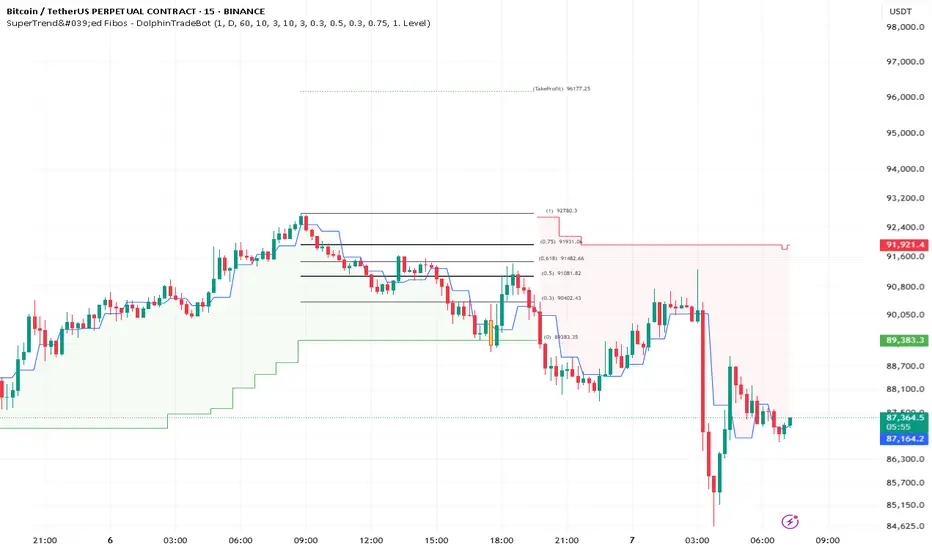
SuperTrend'ed Fibos - DolphinTradeBot
Overwiev
This indicator aims to assist in taking trades at relatively low price levels in the direction of the main trend and capturing profits at potential reversal points.
What is it for !
The indicator simply performs its calculations by using two multitimeframe SuperTrend indicators, Fibonacci levels, and pivot points. The reason for using MTF in both SuperTrend indicators is that the lengths of the levels are relatively limited, so it allows for a more detailed analysis on lower timeframes.
How is it work
When both the HTF SuperTrend and the main SuperTrend indicators are in the same direction,
For Uptrend:
Once the main SuperTrend line is violated it barcolor and draws the basic Fibonacci levels between the pivot high point and the SuperTrend line within the trend region . The TakeProfit level is drawn at a distance multiplied by the TakeProfit Multiplier, between the lowest and highest points of the level. When the main trend reverses or the TakeProfit level is violated, it stops drawing.
For Downtrend:
Once the main SuperTrend line is violated it barcolor and draws the basic Fibonacci levels between the pivot low point and the SuperTrend line within the trend region . The TakeProfit level is drawn at a distance multiplied by the TakeProfit Multiplier, between the lowest and highest points of the level. When the main trend reverses or the TakeProfit level is violated, it stops drawing.
How to Use:
To prevent the line thickness from being displayed on the screen, the indicator shows the direction of the HTF SuperTrend indicator by coloring the background. In the settings section, you can adjust:
TakeProfit Multiplier
Fibonacci line colors
HTF SuperTrend activation
HTF SuperTrend settings
Main SuperTrend settings
Fibonacci levels
Custom alert activation
Custom alert level
Alarm Section
By default, the indicator gives an alert when a level is formed or violated. Additionally, if you want to set an alert for a specific level, you can activate the Custom Alert option and choose your desired level.
Discount/Premium OTE LevelsThis indicator is created to identify discount/premium areas to provide additional confluence to trades taken. The underlying theory is that the trades taken in discounted areas are likely to have less risk due to a smaller stop loss and a higher reward/risk ratio.
The indicator operates by first identifying a zone between the last major swing high and low. These highs and lows are determined as price points that at the extremes within the number of bars to the left, as defined by the "Swing Sensitivity" setting.
Once a price zone is established, the indicator verifies that the zone meets the minimum size in points as configured via the "Minimum size" setting to be considered tradable. Zones that are too small may not provide a sufficient range even for scalping. The default value is 42 points based on Nasdaq, which means that the distance between inner most OTE levels (0.382 and 0.618) is at least 10 points.
When a valid zone is identified, it is then subdivided into areas of interest based on OTE levels, which can be configured/adjusted via the "Levels to Draw" setting. These levels represent the midpoint (50%), which distinguishes between premium and discount, and the three OTE levels 0.79, 0.705, 0.618, above the 50% for discount and below the 50% for premium.
For example, if a zone is formed initially by a swing low followed by a swing high with the assumption that the draw is higher, the indicator can be used to formulate long positions from below the 50% level starting at 0.38 OTE level, or ideally at 0.295 OTE level using 0 as a stop loss. Alternatively, if the 50% level is not yet tapped, short scalp positions can be made from 0.79-0.618 OTE levels with 50% as a partial or TP target.
See for long/short example
Typically, the indicator will show only a single zone. However, there may be cases with two zones: one larger parent zone containing a smaller, valid price zone within itself.
The indicator will automatically invalidate and remove the zone once the high/low of the zone is invalidated.
Configuration:
The indicator provides several visualization options for customization, including:
Color settings for OTE levels, with separate settings for edge/50% color, premium, and discount levels.
Settings for line style for OTE levels.
Settings to determine whether to show prices on level labels.
Settings to decide if lines should be extended to the right.

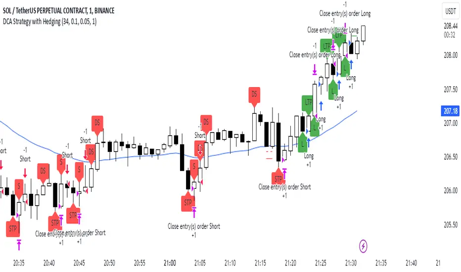
DCA Strategy with HedgingThis strategy implements a dynamic hedging system with Dollar-Cost Averaging (DCA) based on the 34 EMA. It can hold simultaneous long and short positions, making it suitable for ranging and trending markets.
Key Features:
Uses 34 EMA as baseline indicator
Implements hedging with simultaneous long/short positions
Dynamic DCA for position management
Automatic take-profit adjustments
Entry confirmation using 3-candle rule
How it Works
Long Entries:
Opens when price closes above 34 EMA for 3 candles
Adds positions every 0.1% price drop
Takes profit at 0.05% above average entry
Short Entries:
Opens when price closes below 34 EMA for 3 candles
Adds positions every 0.1% price rise
Takes profit at 0.05% below average entry
Settings
EMA Length: Controls the EMA period (default: 34)
DCA Interval: Price movement needed for additional entries (default: 0.1%)
Take Profit: Profit target from average entry (default: 0.05%)
Initial Position: Starting position size (default: 1.0)
Indicators
L: Long Entry
DL: Long DCA
S: Short Entry
DS: Short DCA
LTP: Long Take Profit
STP: Short Take Profit
Alerts
Compatible with all standard TradingView alerts:
Position Opens (Long/Short)
DCA Entries
Take Profit Hits
Note: This strategy works best on lower timeframes with high liquidity pairs. Adjust parameters based on asset volatility.
Ultra Trade JournalThe Ultra Trade Journal is a powerful TradingView indicator designed to help traders meticulously document and analyze their trades. Whether you're a novice or an experienced trader, this tool offers a clear and organized way to visualize your trading strategy, monitor performance, and make informed decisions based on detailed trade metrics.
Detailed Description
The Ultra Trade Journal indicator allows users to input and visualize critical trade information directly on their TradingView charts.
.........
User Inputs
Traders can specify entry and exit prices , stop loss levels, and up to four take profit targets.
.....
Dynamic Plotting
Once the input values are set, the indicator automatically plots horizontal lines for entry, exit, stop loss, and each take profit level on the chart. These lines are visually distinct, using different colors and styles (solid, dashed, dotted) to represent each element clearly.
.....
Live Position Tracking
If enabled, the indicator can adjust the exit price in real-time based on the current market price, allowing traders to monitor live positions effectively.
.....
Tick Calculations
The script calculates the number of ticks between the entry price and each exit point (stop loss and take profits). This helps in understanding the movement required for each target and assessing the potential risk and reward.
.....
Risk-Reward Ratios
For each take profit level, the indicator computes the risk-reward (RR) ratio by comparing the ticks at each target against the stop loss ticks. This provides a quick view of the potential profitability versus the risk taken.
.....
Comprehensive Table Display
A customizable table is displayed on the chart, summarizing all key trade details. This includes the entry and exit prices, stop loss and take profit levels, tick counts, and their respective RR ratios.
Users can adjust the table's Position and text color to suit their preferences.
.....
Visual Enhancements
The indicator uses adjustable background shading between entry and stop loss/take profit lines to visually represent potential trade outcomes. This shading adjusts based on whether the trade is long or short, providing an intuitive understanding of trade performance.
.........
Overall, the Ultra Trade Journal combines visual clarity with detailed analytics, enabling traders to keep a well-organized record of their trades and enhance their trading strategies through insightful data.

ATR% Multiple from Key Moving AverageThis script gives signal when the ATR% multiple from any chosen moving average is beyond the configurable threshold value. This indicator quantifies how extended the stock is from a given key moving average.
A lot of traders use ATR% multiple from 10DMA, 21EMA, 50SMA or 200SMA to determine how extended a stock is and accordingly sell partials or exit. By default the indicator takes 50SMA and when the ATR% multiple is greater than 7 then it gives the signal to take partials. You can back test this indicator with previous trades and determine the ideal threshold for the signal. For small and midcaps a threshold of 7 to 10 ATR% multiples from 50SMA is where partials can be taken while large caps can revert to mean even earlier at 3 to 5 ATR% multiples from 50SMA.
You can modify this script and use it anyway you please as long as you make it opensource on TradingView.

16. SMC Strategy with SL - low TimeframeOverview
The "SMC Strategy with SL - low Timeframe" is a comprehensive trading strategy that uses key concepts from Smart Money Theory to identify favorable areas in the market for buying or selling. This strategy takes advantage of price imbalances, support and resistance zones, and swing highs/lows to generate high-probability trade signals.
The key features of this strategy include:
Swing High/Low Analysis: Used to determine the Premium, Equilibrium, and Discount Zones.
Order Block Integration: An added layer of confluence to identify valid buy and sell signals.
Trend Direction Confirmation: Using a Simple Moving Average (SMA) to determine the overall trend.
Entry and Exit Rules: Based on price position relative to key zones and moving average, along with optional stop-loss and take-profit levels.
Detailed Description
Swing High and Swing Low Analysis
The script calculates Swing High and Swing Low based on the most recent price highs and lows over a specified look-back period (swingHighLength and swingLowLength, set to 8 by default).
It then derives the Premium, Equilibrium, and Discount Zones:
Premium Zone: Represents potential resistance, calculated based on recent swing highs.
Discount Zone: Represents potential support, calculated based on recent swing lows.
Equilibrium: The midpoint between Swing High and Swing Low, dividing the price range into Premium (above equilibrium) and Discount (below equilibrium) areas.
Zone Visualization
The strategy plots the Premium Zone (resistance) in red, the Discount Zone (support) in green, and the Equilibrium level in blue on the chart. This helps visually assess the current price relative to these important areas.
Simple Moving Average (SMA)
A 50-period Simple Moving Average (SMA) is added to help identify the trend direction.
Buy signals are valid only if the price is above the SMA, indicating an uptrend.
Sell signals are valid only if the price is below the SMA, indicating a downtrend.
Entry Rules
The script generates buy or sell signals when certain conditions are met:
A buy signal is triggered when:
Price is below the Equilibrium and within the Discount Zone.
Price is above the SMA.
The buy signal is further confirmed by the presence of an Order Block (recent lowest price area).
A sell signal is triggered when:
Price is above the Equilibrium and within the Premium Zone.
Price is below the SMA.
The sell signal is further confirmed by the presence of an Order Block (recent highest price area).
Order Block
The strategy defines Order Blocks as recent highs and lows within a look-back period (orderBlockLength set to 20 by default).
These blocks represent areas where large players (smart money) have historically been active, increasing the probability of the price reacting in these areas again.
Trade Management and Trade Direction
The user can set Trade Direction to either "Long Only," "Short Only," or "Both." This allows the strategy to adapt based on market conditions or trading preferences.
Based on the Trade Direction, the strategy either:
Closes open trades that are against new signals.
Allows only specific directional trades (either long or short).
Stop-loss levels are defined based on a fixed percentage (stop_loss_percent), which helps to manage risk and minimize losses.
Exit Rules
The strategy uses stop-loss levels for risk management.
A stop-loss price is set at a fixed percentage below the entry price for long positions or above the entry price for short positions.
When the price hits the defined stop-loss level, the trade is closed.
Liquidity Zones
The script identifies recent Swing Highs and Lows as potential liquidity zones. These are levels where price could react strongly, as they represent areas of interest for large traders.
The liquidity zones are plotted as crosses on the chart, marking areas where price may encounter significant buying or selling pressure.
Visual Feedback
The script uses visual markers (green for buy signals and red for sell signals) to indicate potential entries on the chart.
It also plots liquidity zones to help traders identify areas where stop hunts and liquidity grabs might occur.
Monthly Performance Dashboard
The script includes a performance tracking feature that displays monthly profit and loss metrics on the chart.
This dashboard allows the trader to see a visual representation of trading performance over time, providing insights into profitability and consistency.
The table shows profit or loss for each month and year, allowing the user to track the overall success of the strategy.
Key Benefits
Smart Money Concepts (SMC): This strategy incorporates SMC principles like order blocks and liquidity zones, which are used by institutional traders to determine potential market moves.
Zone Analysis: The use of Premium, Discount, and Equilibrium zones provides a solid framework for determining where to enter and exit trades based on price discounts or premiums.
Confluence: Signals are not taken in isolation. They are confirmed by factors like trend direction (SMA) and order blocks, providing greater trade accuracy.
Risk Management: By integrating stop-loss functionality, traders can manage their risks effectively.
Visual Performance Metrics: The monthly and yearly performance dashboard gives valuable feedback on how well the strategy has performed historically.
Practical Use
Buy in Discount Zone: Traders would be looking to buy when the price is discounted relative to its recent range and is above the SMA, indicating an overall uptrend.
Sell in Premium Zone: Conversely, traders would be looking to sell when the price is at a premium relative to its recent range and below the SMA, indicating an overall downtrend.
Order Block Confirmation: Ensures that buying or selling is supported by historical price behavior at significant levels, providing confidence that the market is likely to react at these areas.
This strategy is designed to help traders take advantage of price inefficiencies and areas where institutional traders are likely to be active, increasing the odds of successful trades. By leveraging Smart Money concepts and strong technical confluence, it aims to provide high-probability trade setups.

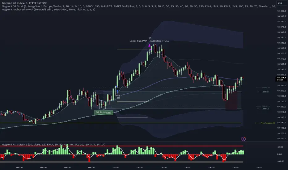
Negroni Opening Range StrategyStrategy Summary:
This tool can be used to help identify breakouts from a range during a time-zone of your choosing. It plots a pre-market range, an opening range, it also includes moving average levels that can be used as confluence, as well as plotting previous day SESSION highs and lows.
There are several options on how you wish to close out the trades, all described in more detail below.
Back-testing Inputs:
You define your timezone.
You define how many trades to open on any given day.
You decide to go: long only, short only, or long & short (CAREFUL: "Long & Short" can open trades that effectively closes-out existing ones, for better AND worse!)
You define between which times the strategy will open trades.
You define when it closes any open trades (preventing overnight trades, or leaving trades open into US data times!!).
This hopefully helps make back-testing reflect YOUR trading hours.
NOTE: Renko or Heikin-Ashi charts
For ALL strategies, don’t use Renko or Heikin-Ashi charts unless you know EXACTLY the implications.
Specific to my strategy, using a renko chart can make this 85-90% profitable (I wish it was!!) Although they can be useful, renko charts don’t always capture real wicks, so the renko chart may show your trade up-only but your broker (who is not using renko!!) will have likely stopped you out on a wick somewhere along the line.
NOTE: TradingView ‘Deep backtesting’
For ALL strategies, be cynical of all backtesting (e.g. repainting issues etc) as well as ‘Deep backtesting’ results.
Specific to this strategy, the default settings here SHOULD BE OK, but unfortunately at the time of writing, we can’t see on the chart what exactly ‘deep backtesting’ is calculating. In the past I have noted a number of trades that were not closed at the end of the day, despite my ‘end of day’ trade closing being enabled, so there were big winners and losers that would not have materialized otherwise. As I say, this seems ok at these settings but just always be cynical!!
Opening Range Inputs
You define a pre-market range (example: 08:00 - 09:00).
You define an opening range (example: 09:00 - 09:30).
The strategy will give an update at the close of the opening range to let you know if the opening range has broken out the pre-market range (OR Breakout), or if it has remained inside (OR Inside). The label appears at the end of the opening range NOT at the bar that ‘broke-out’.
This is just a visual cue for you, it has no bearing on what the strategy will do.
The strategy default will trade off the pre-market range, but you can untick this if you prefer to trade off the opening range.
Opening Trades:
Strategy goes long when the bar (CLOSE) crosses-over the ‘pre-market’ high (not the ‘opening range’ high); and the time is within your trading session, and you have not maxed out your number of trades for the day!
Strategy goes short when the bar (CLOSE) crosses-under the ‘pre-market’ low (not the ‘opening range low); and the time is within your trading session, and you have not maxed out your number of trades for the day!
Remember, you can untick this if you prefer to trade off the opening range instead.
NOTES:
Using momentum indicators can help (RSI and MACD): especially to trade range plays in failed breakouts, when momentum shifts… but the strategy won’t do this for you!
Using an anchored vwap at the session open can also provide nice confluence, as well as take-profit levels at the upper/lower of 3x standard deviation.
CLOSING TRADES:
You have 6 take-profit (TP) options:
1) Full TP: uses ATR Multiplier - Full TP at the ATR parameters as defined in inputs.
2) Take Partial profits: ATR Multiplier - Takes partial profits based on parameters as defined in inputs (i.e close 40% of original trade at TP1, close another 40% of original trade at TP2, then the remainder at Full TP as set in option 1.).
3) Full TP: Trailing Stop - Applies a Trailing Stop at the number of points, as defined in inputs.
4) Full TP: MA cross - Takes profit when price crosses ‘Trend MA’ as defined in inputs.
5) Scalp: Points - closes at a set number of points, as defined in inputs.
6) Full TP: PMKT Multiplier - places a SL at opposite pre-market Hi/Low (we go long at a break-out of the pre-market high, 50% would place a SL at the pre-market range mid-point; 100% would place a SL at the pre-market low)'. This takes profit at the input set in option 1).
BBTrend w SuperTrend decision - Strategy [presentTrading]This strategy aims to improve upon the performance of Traidngview's newly published "BB Trend" indicator by incorporating the SuperTrend for better trade execution and risk management. Enjoy :)
█Introduction and How it is Different
The "BBTrend w SuperTrend decision - Strategy " is a trading strategy designed to identify market trends using Bollinger Bands and SuperTrend indicators. What sets this strategy apart is its use of two Bollinger Bands with different lengths to capture both short-term and long-term market trends, providing a more comprehensive view of market dynamics. Additionally, the strategy includes customizable take profit (TP) and stop loss (SL) settings, allowing traders to tailor their risk management according to their preferences.
BTCUSD 4h Long Performance
█ Strategy, How It Works: Detailed Explanation
The BBTrend strategy employs two key indicators: Bollinger Bands and SuperTrend.
🔶 Bollinger Bands Calculation:
- Short Bollinger Bands**: Calculated using a shorter period (default 20).
- Long Bollinger Bands**: Calculated using a longer period (default 50).
- Bollinger Bands use the standard deviation of price data to create upper and lower bands around a moving average.
Upper Band = Middle Band + (k * Standard Deviation)
Lower Band = Middle Band - (k * Standard Deviation)
🔶 BBTrend Indicator:
- The BBTrend indicator is derived from the absolute differences between the short and long Bollinger Bands' lower and upper values.
BBTrend = (|Short Lower - Long Lower| - |Short Upper - Long Upper|) / Short Middle * 100
🔶 SuperTrend Indicator:
- The SuperTrend indicator is calculated using the average true range (ATR) and a multiplier. It helps identify the market trend direction by plotting levels above and below the price, which act as dynamic support and resistance levels. * @EliCobra makes the SuperTrend Toolkit. He is GOAT.
SuperTrend Upper = HL2 + (Factor * ATR)
SuperTrend Lower = HL2 - (Factor * ATR)
The strategy determines market trends by checking if the close price is above or below the SuperTrend values:
- Uptrend: Close price is above the SuperTrend lower band.
- Downtrend: Close price is below the SuperTrend upper band.
Short: 10 Long: 20 std 2
Short: 20 Long: 40 std 2
Short: 20 Long: 40 std 4
█ Trade Direction
The strategy allows traders to choose their trading direction:
- Long: Enter long positions only.
- Short: Enter short positions only.
- Both: Enter both long and short positions based on market conditions.
█ Usage
To use the "BBTrend - Strategy " effectively:
1. Configure Inputs: Adjust the Bollinger Bands lengths, standard deviation multiplier, and SuperTrend settings.
2. Set TPSL Conditions: Choose the take profit and stop loss percentages to manage risk.
3. Choose Trade Direction: Decide whether to trade long, short, or both directions.
4. Apply Strategy: Apply the strategy to your chart and monitor the signals for potential trades.
█ Default Settings
The default settings are designed to provide a balance between sensitivity and stability:
- Short BB Length (20): Captures short-term market trends.
- Long BB Length (50): Captures long-term market trends.
- StdDev (2.0): Determines the width of the Bollinger Bands.
- SuperTrend Length (10): Period for calculating the ATR.
- SuperTrend Factor (12): Multiplier for the ATR to adjust the SuperTrend sensitivity.
- Take Profit (30%): Sets the level at which profits are taken.
- Stop Loss (20%): Sets the level at which losses are cut to manage risk.
Effect on Performance
- Short BB Length: A shorter length makes the strategy more responsive to recent price changes but can generate more false signals.
- Long BB Length: A longer length provides smoother trend signals but may be slower to react to price changes.
- StdDev: Higher values create wider bands, reducing the frequency of signals but increasing their reliability.
- SuperTrend Length and Factor: Shorter lengths and higher factors make the SuperTrend more sensitive, providing quicker signals but potentially more noise.
- Take Profit and Stop Loss: Adjusting these levels affects the risk-reward ratio. Higher take profit percentages can increase gains but may result in fewer closed trades, while higher stop loss percentages can decrease the likelihood of being stopped out but increase potential losses.

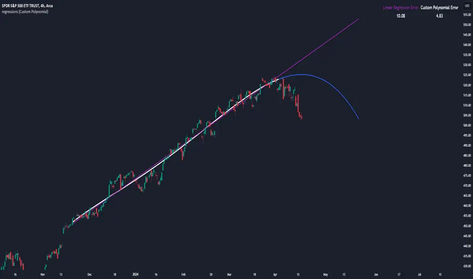
regressionsLibrary "regressions"
This library computes least square regression models for polynomials of any form for a given data set of x and y values.
fit(X, y, reg_type, degrees)
Takes a list of X and y values and the degrees of the polynomial and returns a least square regression for the given polynomial on the dataset.
Parameters:
X (array) : (float ) X inputs for regression fit.
y (array) : (float ) y outputs for regression fit.
reg_type (string) : (string) The type of regression. If passing value for degrees use reg.type_custom
degrees (array) : (int ) The degrees of the polynomial which will be fit to the data. ex: passing array.from(0, 3) would be a polynomial of form c1x^0 + c2x^3 where c2 and c1 will be coefficients of the best fitting polynomial.
Returns: (regression) returns a regression with the best fitting coefficients for the selecected polynomial
regress(reg, x)
Regress one x input.
Parameters:
reg (regression) : (regression) The fitted regression which the y_pred will be calulated with.
x (float) : (float) The input value cooresponding to the y_pred.
Returns: (float) The best fit y value for the given x input and regression.
predict(reg, X)
Predict a new set of X values with a fitted regression. -1 is one bar ahead of the realtime
Parameters:
reg (regression) : (regression) The fitted regression which the y_pred will be calulated with.
X (array)
Returns: (float ) The best fit y values for the given x input and regression.
generate_points(reg, x, y, left_index, right_index)
Takes a regression object and creates chart points which can be used for plotting visuals like lines and labels.
Parameters:
reg (regression) : (regression) Regression which has been fitted to a data set.
x (array) : (float ) x values which coorispond to passed y values
y (array) : (float ) y values which coorispond to passed x values
left_index (int) : (int) The offset of the bar farthest to the realtime bar should be larger than left_index value.
right_index (int) : (int) The offset of the bar closest to the realtime bar should be less than right_index value.
Returns: (chart.point ) Returns an array of chart points
plot_reg(reg, x, y, left_index, right_index, curved, close, line_color, line_width)
Simple plotting function for regression for more custom plotting use generate_points() to create points then create your own plotting function.
Parameters:
reg (regression) : (regression) Regression which has been fitted to a data set.
x (array)
y (array)
left_index (int) : (int) The offset of the bar farthest to the realtime bar should be larger than left_index value.
right_index (int) : (int) The offset of the bar closest to the realtime bar should be less than right_index value.
curved (bool) : (bool) If the polyline is curved or not.
close (bool) : (bool) If true the polyline will be closed.
line_color (color) : (color) The color of the line.
line_width (int) : (int) The width of the line.
Returns: (polyline) The polyline for the regression.
series_to_list(src, left_index, right_index)
Convert a series to a list. Creates a list of all the cooresponding source values
from left_index to right_index. This should be called at the highest scope for consistency.
Parameters:
src (float) : (float ) The source the list will be comprised of.
left_index (int) : (float ) The left most bar (farthest back historical bar) which the cooresponding source value will be taken for.
right_index (int) : (float ) The right most bar closest to the realtime bar which the cooresponding source value will be taken for.
Returns: (float ) An array of size left_index-right_index
range_list(start, stop, step)
Creates an from the start value to the stop value.
Parameters:
start (int) : (float ) The true y values.
stop (int) : (float ) The predicted y values.
step (int) : (int) Positive integer. The spacing between the values. ex: start=1, stop=6, step=2:
Returns: (float ) An array of size stop-start
regression
Fields:
coeffs (array__float)
degrees (array__float)
type_linear (series__string)
type_quadratic (series__string)
type_cubic (series__string)
type_custom (series__string)
_squared_error (series__float)
X (array__float)
Open Liquidity Heatmap [BigBeluga]Open Liquidity Heatmap is an indicator designed to display accumulated resting liquidity on the chart.
Unlike any other liquidity heatmap, this aims to accumulate liquidity at specific levels that build up over time, showing larger areas of liquidity.
🔶 FEATURES
The indicator includes the following settings:
Lookback : Used to determine the range calculation of the heatmap.
Leverage : Leverage of the liquidation (Counted as % in price, Example: 4.5 will return a distance from price of 4.5%, indicating any possible resting liquidity in this range).
Levels : Amount of levels to display (Each level is counted as liquidity resting on the chart; fewer levels will return a bigger area of liquidity sitting on the chart).
Mode : Apply a color gradient from the minimum liquidation to the maximum liquidity level. Set the maximum color gradient value (Counted as volume).
Offset : Automatically determine the offset range of the Volume Profiles. Manual offset of the Volume Profiles.
🔶 CALCULATION
for i = 0 to step - 1
float plotter = na
switch i
0 =>
plotter := hs
=>
plotter := hs - diff * ( i )
cls.hm.gnL(plotter)
cls.vp.put(plotter, 0)
We calculate levels like a normal volume profile with steps, from the highest point within the lookback to the lowest one. Each level will contain the corresponding amount of volume that the candle has closed in that range.
As we can see in the image above, we add liquidity each time the distance in % from price is between two levels.
Unlike many liquidity indicators that provide a single candle liquidity heatmap, this aims to add up liquidity (volume) in already present levels.
This can be extremely useful to see which levels are likely to be more liquid and tend to get a bigger reaction to the price.
Imagine it like a range of levels that each time price revisits that area, a new position area is added; we add volume in that area each time price visits that zone. Liquidity builds up in those zones, causing a bigger reaction to the price once the price visits it.
This indicator is not the same as a single candle heatmap like many others. What is a single candle heatmap?
A single candle heatmap is when a level is created on every new candle, coloring the level based on the total volume of it.
This indicator, on the contrary, aims to provide a more specific use by adding up liquidity each time price visits it.
🔶 BASIC DEMOSTRATION
This is a basic demonstration of how we can spot high liquidity points overall using confluence:
We see the POC of the liquidation in a low volume area of the normal volume profile adding up as confluence.
Resistance from the POC Volume Profile suggesting price will go lower.
Major long open liquidity down.
As we can see, price takes out all the long liquidity and right after pumping, indicating that all the major liquidity got taken out.
Some key note to take is that a POC in the liquidation heatmap in a low volume area of the normal Volume Profile add confluence of a possible big reaction in that zone.
In the forex market, we suggest to use a low distance from price (Leverage) while in a crypto market you can use the one that fit the best the current timeframe.
🔶 CONCLUSION
This indicator aims to show open resting liquidity that had built up over time, showing the most amount of liquidation in specific areas in an aggregated way unlike many liquidation heatmap indicators that show single-level liquidation.
🔶 RELATED SCRIPT

Optimal Buy Day (Zeiierman)█ Overview
The Optimal Buy Day (Zeiierman) indicator identifies optimal buying days based on historical price data, starting from a user-defined year. It simulates investing a fixed initial capital and making regular monthly contributions. The unique aspect of this indicator involves comparing systematic investment on specific days of the month against a randomized buying day each month, aiming to analyze which method might yield more shares or a better average price over time. By visualizing the potential outcomes of systematic versus randomized buying, traders can better understand the impact of market timing and how regular investments might accumulate over time.
These statistics are pivotal for traders and investors using the script to analyze historical performance and strategize future investments. By understanding which days offered more shares for their money or lower average prices, investors can tailor their buying strategies to potentially enhance returns.
█ Key Statistics
⚪ Shares
Definition: Represents the total number of shares acquired on a particular day of the month across the entire simulation period.
How It Works: The script calculates how many shares can be bought each day, given the available capital or monthly contribution. This calculation takes into account the day's opening price and accumulates the total shares bought on that day over the simulation period.
Interpretation: A higher number of shares indicates that the day consistently offered better buying opportunities, allowing the investor to acquire more shares for the same amount of money. This metric is crucial for understanding which days historically provided more value.
⚪ AVG Price
Definition: The average price paid per share on a particular day of the month, averaged over the simulation period.
How It Works: Each time shares are bought, the script calculates the average price per share, factoring in the new shares purchased at the current price. This average evolves over time as more shares are bought at varying prices.
Interpretation: The average price gives insight into the cost efficiency of buying shares on specific days. A lower average price suggests that buying on that day has historically led to better pricing, making it a potentially more attractive investment strategy.
⚪ Buys
Definition: The total number of transactions or buys executed on a particular day of the month throughout the simulation.
How It Works: This metric increments each time shares are bought on a specific day, providing a count of all buying actions taken.
Interpretation: The number of buys indicates the frequency of investment opportunities. A higher count could mean more consistent opportunities for investment, but it's important to consider this in conjunction with the average price and the total shares acquired to assess overall strategy effectiveness.
⚪ Most Shares
Definition: Identifies the day of the month on which the highest number of shares were bought, highlighting the specific day and the total shares acquired.
How It Works: After simulating purchases across all days of the month, the script identifies which day resulted in the highest total number of shares bought.
Interpretation: This metric points out the most opportune day for volume buying. It suggests that historically, this day provided conditions that allowed for maximizing the quantity of shares purchased, potentially due to lower prices or other factors.
⚪ Best Price
Definition: Highlights the day of the month that offered the lowest average price per share, indicating both the day and the price.
How It Works: The script calculates the average price per share for each day and identifies the day with the lowest average.
Interpretation: This metric is key for investors looking to minimize costs. The best price day suggests that historically, buying on this day led to acquiring shares at a more favorable average price, potentially maximizing long-term investment returns.
⚪ Randomized Shares
Definition: This metric represents the total number of shares acquired on a randomly selected day of the month, simulated across the entire period.
How It Works: At the beginning of each month within the simulation, the script selects a random day when the market is open and calculates how many shares can be purchased with the available capital or monthly contribution at that day's opening price. This process is repeated each month, and the total number of shares acquired through these random purchases is tallied.
Interpretation: Randomized shares offer a comparison point to systematic buying strategies. By comparing the total shares acquired through random selection against those bought on the best or worst days, investors can gauge the impact of timing and market fluctuations on their investment strategy. A higher total in randomized shares might indicate that over the long term, the specific days chosen for investment might matter less than consistent market participation. Conversely, if systematic strategies yield significantly more shares, it suggests that timing could indeed play a crucial role in maximizing investment returns.
⚪ Randomized Price
Definition: The average price paid per share for the shares acquired on the randomly selected days throughout the simulation period.
How It Works: Each time shares are bought on a randomly chosen day, the script calculates the average price paid for all shares bought through this randomized strategy. This average price is updated as the simulation progresses, reflecting the cost efficiency of random buying decisions.
Interpretation: The randomized price metric helps investors understand the cost implications of a non-systematic, random investment approach. Comparing this average price to those achieved through more deliberate, systematic strategies can reveal whether consistent investment timing strategies outperform random investment actions in terms of cost efficiency. A lower randomized price suggests that random buying might not necessarily result in higher costs, while a higher average price indicates that systematic strategies might provide better control over investment costs.
█ How to Use
Traders can use this tool to analyze historical data and simulate different investment strategies. By inputting their initial capital, regular contribution amount, and start year, they can visually assess which days might have been more advantageous for buying, based on historical price actions. This can inform future investment decisions, especially for those employing dollar-cost averaging strategies or looking to optimize entry points.
█ Settings
StartYear: This setting allows the user to specify the starting year for the investment simulation. Changing this value will either extend or shorten the period over which the simulation is run. If a user increases the value, the simulation begins later and covers a shorter historical period; decreasing the value starts the simulation earlier, encompassing a longer time frame.
Capital: Determines the initial amount of capital with which the simulation begins. Increasing this value simulates starting with more capital, which can affect the number of shares that can be initially bought. Decreasing this value simulates starting with less capital.
Contribution: Sets the monthly financial contribution added to the investment within the simulation. A higher contribution increases the investment each month and could lead to more shares being purchased over time. Lowering the contribution decreases the monthly investment amount.
-----------------
Disclaimer
The information contained in my Scripts/Indicators/Ideas/Algos/Systems does not constitute financial advice or a solicitation to buy or sell any securities of any type. I will not accept liability for any loss or damage, including without limitation any loss of profit, which may arise directly or indirectly from the use of or reliance on such information.
All investments involve risk, and the past performance of a security, industry, sector, market, financial product, trading strategy, backtest, or individual's trading does not guarantee future results or returns. Investors are fully responsible for any investment decisions they make. Such decisions should be based solely on an evaluation of their financial circumstances, investment objectives, risk tolerance, and liquidity needs.
My Scripts/Indicators/Ideas/Algos/Systems are only for educational purposes!

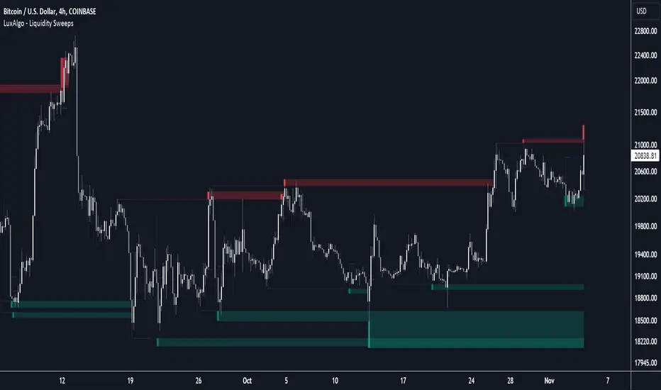
Liquidity Sweeps [LuxAlgo]The Liquidity Sweeps indicator detects the presence of liquidity sweeps on the user's chart, while also providing potential areas of support/resistance or entry when Liquidity levels are taken.
In the event of a Liquidity Sweep a Sweep Area is created which may provide further areas of interest.
🔶 USAGE
A Liquidity Sweep occurs when the price breaks through a liquidity level (further referred to as LqL ), after which the price returns below/above the liquidity level , forming a wick.
The script provides 2 options when this can happen:
A wick passes a LqL after which the price quickly returns.
First the closing price breaks through a LqL . After a while, the price retests the LqL and forms a wick in the opposite direction.
The examples above show a bullish and bearish scenario of "a wick passing through an LqL where the price quickly comes back". This type of Liquidity Sweep is represented by a dotted line.
The following example shows a broken LqL , where the price retests the Liquidity zone and bounces back.
Instead of a dotted line, this type of Liquidity Sweep is represented by a dashed line.
When a Liquidity Sweep takes place, this is indicated by highlighting the "wick- LqL " distance. This distance is also the basis for the Sweep Area (see next sub-section). A small 3-bar long dotted line starts from the opposite wick as an extra aid to determine potential support/resistance/entry, ...
Colors can be set in the settings (here yellow and aqua blue instead of default colors for clarity).
🔹 Sweep Areas
The distance between the LqL and the maximum limit of the wick forms a Sweep Area , which can provide a potential support/resistance or entry zone.
These examples show both types of Liquidity Sweeps , followed by a box indicating the Sweep Area .
When the Sweep Area is mitigated or a certain amount of bars has passed (Settings - 'Max bars'), the boxes will no longer be updated.
In this case, the 'Trigger' label shows the bar where the high crossed a LqL , after which a red box starts between LqL and high.
The low of the 'Trigger' bar is the starting point of a short dotted line. Next to the 'Trigger bar' the high touches the Sweep Area before returning, providing a potential short entry. One bar further, another entry opportunity presents itself when the price breaks the small dotted line.
In the following bullish example, not only do we see opportunities when the LqL has been swept, but the following Sweep Area provides some potential entries.
The small green dotted lines also act as a guide where the price breaks above, then forms a small range, after which the price continues in an upward direction.
Here, the initial trigger on the left forms a Sweep Area that is quickly broken. However, the small green line provides a potential entry area later on. The price moves in a short channel before breaking above the LqL (green dashed line), providing more potential entries. Price retests this LqL , and goes below this level. The price remained around the previously formed channel, after which the price resumed its upward trend.
🔶 SETTINGS
🔹 Liquidity Sweeps
Swings: Period used for the swing detection, with higher values returning longer term Liquidity Levels .
Options:
- Only Wicks: Only detects a Liquidity Sweep when a wick sweeps a previous wick
- Only Outbreaks & Retest: Only detects a Liquidity Sweep when the price breaks a Liquidity Level , returns & retests the Liquidity Level , and forms a wick in the opposite direction.
- Wicks + Outbreaks & Retest: Both options can be detected.
🔹 Sweep Area
Extend: Enables/Disables extension of the Sweep Area boxes.
Max Bars: Limit the extension to a certain number of bars.
Color Sweep Area box.
Triple Confirmation Kernel Regression Overlay [QuantraSystems]Kernel Regression Oscillator - Overlay
Introduction
The Kernel Regression Oscillator (ᏦᏒᎧ) represents an advanced tool for traders looking to capitalize on market trends.
This Indicator is valuable in identifying and confirming trend directions, as well as probabilistic and dynamic oversold and overbought zones.
It achieves this through a unique composite approach using three distinct Kernel Regressions combined in an Oscillator.
The additional Chart Overlay Indicator adds confidence to the signal.
Which is this Indicator.
This methodology helps the trader to significantly reduce false signals and offers a more reliable indication of market movements than more widely used indicators can.
Legend
The upper section is the Overlay. It features the Signal Wave to display the current trend.
Its Overbought and Oversold zones start at 50% and end at 100% of the selected Standard Deviation (default σ = 3), which can indicate extremely rare situations which can lead to either a softening momentum in the trend or even a mean reversion situation.
The lower one is the Base Chart.
The Indicator is linked here
It features the Kernel Regression Oscillator to display a composite of three distinct regressions, also displaying current trend.
Its Overbought and Oversold zones start at 50% and end at 100% of the selected Standard Deviation (default σ = 2), which can indicate extremely rare situations.
Case Study
To effectively utilize the ᏦᏒᎧ, traders should use both the additional Overlay and the Base
Chart at the same time. Then focus on capturing the confluence in signals, for example:
If the 𝓢𝓲𝓰𝓷𝓪𝓵 𝓦𝓪𝓿𝓮 on the Overlay and the ᏦᏒᎧ on the Base Chart both reside near the extreme of an Oversold zone the probability is higher than normal that momentum in trend may soften or the token may even experience a reversion soon.
If a bar is characterized by an Oversold Shading in both the Overlay and the Base Chart, then the probability is very high to experience a reversion soon.
In this case the trader may want to look for appropriate entries into a long position, as displayed here.
If a bar is characterized by an Overbought Shading in either Overlay or Base Chart, then the probability is high for momentum weakening or a mean reversion.
In this case the trade may have taken profit and closed his long position, as displayed here.
Please note that we always advise to find more confluence by additional indicators.
Recommended Settings
Swing Trading (1D chart)
Overlay
Bandwith: 45
Width: 2
SD Lookback: 150
SD Multiplier: 2
Base Chart
Bandwith: 45
SD Lookback: 150
SD Multiplier: 2
Fast-paced, Scalping (4min chart)
Overlay
Bandwith: 75
Width: 2
SD Lookback: 150
SD Multiplier: 3
Base Chart
Bandwith: 45
SD Lookback: 150
SD Multiplier: 2
Notes
The Kernel Regression Oscillator on the Base Chart is also sensitive to divergences if that is something you are keen on using.
For maximum confluence, it is recommended to use the indicator both as a chart overlay and in its Base Chart.
Please pay attention to shaded areas with Standard Deviation settings of 2 or 3 at their outer borders, and consider action only with high confidence when both parts of the indicator align on the same signal.
This tool shows its best performance on timeframes lower than 4 hours.
Traders are encouraged to test and determine the most suitable settings for their specific trading strategies and timeframes.
The trend following functionality is indicated through the "𝓢𝓲𝓰𝓷𝓪𝓵 𝓦𝓪𝓿𝓮" Line, with optional "Up" and "Down" arrows to denote trend directions only (toggle “Show Trend Signals”).
Methodology
The Kernel Regression Oscillator takes three distinct kernel regression functions,
used at similar weight, in order to calculate a balanced and smooth composite of the regressions. Part of it are:
The Epanechnikov Kernel Regression: Known for its efficiency in smoothing data by assigning less weight to data points further away from the target point than closer data points, effectively reducing variance.
The Wave Kernel Regression: Similarly assigning weight to the data points based on distance, it captures repetitive and thus wave-like patterns within the data to smoothen out and reduce the effect of underlying cyclical trends.
The Logistic Kernel Regression: This uses the logistic function in order to assign weights by probability distribution on the distance between data points and target points. It thus avoids both bias and variance to a certain level.
kernel(source, bandwidth, kernel_type) =>
switch kernel_type
"Epanechnikov" => math.abs(source) <= 1 ? 0.75 * (1 - math.pow(source, 2)) : 0.0
"Logistic" => 1/math.exp(source + 2 + math.exp(-source))
"Wave" => math.abs(source) <= 1 ? (1 - math.abs(source)) * math.cos(math.pi * source) : 0.
kernelRegression(src, bandwidth, kernel_type) =>
sumWeightedY = 0.
sumKernels = 0.
for i = 0 to bandwidth - 1
base = i*i/math.pow(bandwidth, 2)
kernel = kernel(base, 1, kernel_type)
sumWeightedY += kernel * src
sumKernels += kernel
(src - sumWeightedY/sumKernels)/src
// Triple Confirmations
Ep = kernelRegression(source, bandwidth, 'Epanechnikov' )
Lo = kernelRegression(source, bandwidth, 'Logistic' )
Wa = kernelRegression(source, bandwidth, 'Wave' )
By combining these regressions in an unbiased average, we follow our principle of achieving confluence for a signal or a decision, by stacking several edges to increase the probability that we are correct.
// Average
AV = math.avg(Ep, Lo, Wa)
The Standard Deviation bands take defined parameters from the user, in this case sigma of ideally between 2 to 3,
to help the indicator detect extremely improbable conditions and thus take an inversely probable signal from it to forward to the user.
The parameter settings and also the visualizations allow for ample customizations by the trader. The indicator comes with default and recommended settings.
For questions or recommendations, please feel free to seek contact in the comments.

Triple Confirmation Kernel Regression Base [QuantraSystems]Kernel Regression Oscillator - BASE
Introduction
The Kernel Regression Oscillator (ᏦᏒᎧ) represents an advanced tool for traders looking to capitalize on market trends.
This Indicator is valuable in identifying and confirming trend directions, as well as probabilistic and dynamic oversold and overbought zones.
It achieves this through a unique composite approach using three distinct Kernel Regressions combined in an Oscillator. The additional Chart Overlay Indicator adds confidence to the signal.
This methodology helps the trader to significantly reduce false signals and offers a more reliable indication of market movements than more widely used indicators can.
Legend
The upper section is the Overlay. It features the Signal Wave to display the current trend.
Its Overbought and Oversold zones start at 50% and end at 100% of the selected Standard Deviation (default σ = 3), which can indicate extremely rare situations which can lead to either a softening momentum in the trend or even a mean reversion situation.
The lower one is the Base Chart - This Indicator.
It features the Kernel Regression Oscillator to display a composite of three distinct regressions, also displaying current trend.
Its Overbought and Oversold zones start at 50% and end at 100% of the selected Standard Deviation (default σ = 2), which can indicate extremely rare situations.
Case Study
To effectively utilize the ᏦᏒᎧ, traders should use both the additional Overlay and the Base
Chart at the same time. Then focus on capturing the confluence in signals, for example:
If the 𝓢𝓲𝓰𝓷𝓪𝓵 𝓦𝓪𝓿𝓮 on the Overlay and the ᏦᏒᎧ on the Base Chart both reside near the extreme of an Oversold zone the probability is higher than normal that momentum in trend may soften or the token may even experience a reversion soon.
If a bar is characterized by an Oversold Shading in both the Overlay and the Base Chart, then the probability is very high to experience a reversion soon.
In this case the trader may want to look for appropriate entries into a long position, as displayed here.
If a bar is characterized by an Overbought Shading in either Overlay or Base Chart, then the probability is high for momentum weakening or a mean reversion.
In this case the trade may have taken profit and closed his long position, as displayed here.
Please note that we always advise to find more confluence by additional indicators.
Recommended Settings
Swing Trading (1D chart)
Overlay
Bandwith: 45
Width: 2
SD Lookback: 150
SD Multiplier: 2
Base Chart
Bandwith: 45
SD Lookback: 150
SD Multiplier: 2
Fast-paced, Scalping (4min chart)
Overlay
Bandwith: 75
Width: 2
SD Lookback: 150
SD Multiplier: 3
Base Chart
Bandwith: 45
SD Lookback: 150
SD Multiplier: 2
Notes
The Kernel Regression Oscillator on the Base Chart is also sensitive to divergences if that is something you are keen on using.
For maximum confluence, it is recommended to use the indicator both as a chart overlay and in its Base Chart.
Please pay attention to shaded areas with Standard Deviation settings of 2 or 3 at their outer borders, and consider action only with high confidence when both parts of the indicator align on the same signal.
This tool shows its best performance on timeframes lower than 4 hours.
Traders are encouraged to test and determine the most suitable settings for their specific trading strategies and timeframes.
The trend following functionality is indicated through the "𝓢𝓲𝓰𝓷𝓪𝓵 𝓦𝓪𝓿𝓮" Line, with optional "Up" and "Down" arrows to denote trend directions only (toggle “Show Trend Signals”).
Methodology
The Kernel Regression Oscillator takes three distinct kernel regression functions,
used at similar weight, in order to calculate a balanced and smooth composite of the regressions. Part of it are:
The Epanechnikov Kernel Regression: Known for its efficiency in smoothing data by assigning less weight to data points further away from the target point than closer data points, effectively reducing variance.
The Wave Kernel Regression: Similarly assigning weight to the data points based on distance, it captures repetitive and thus wave-like patterns within the data to smoothen out and reduce the effect of underlying cyclical trends.
The Logistic Kernel Regression: This uses the logistic function in order to assign weights by probability distribution on the distance between data points and target points. It thus avoids both bias and variance to a certain level.
kernel(source, bandwidth, kernel_type) =>
switch kernel_type
"Epanechnikov" => math.abs(source) <= 1 ? 0.75 * (1 - math.pow(source, 2)) : 0.0
"Logistic" => 1/math.exp(source + 2 + math.exp(-source))
"Wave" => math.abs(source) <= 1 ? (1 - math.abs(source)) * math.cos(math.pi * source) : 0.
kernelRegression(src, bandwidth, kernel_type) =>
sumWeightedY = 0.
sumKernels = 0.
for i = 0 to bandwidth - 1
base = i*i/math.pow(bandwidth, 2)
kernel = kernel(base, 1, kernel_type)
sumWeightedY += kernel * src
sumKernels += kernel
(src - sumWeightedY/sumKernels)/src
// Triple Confirmations
Ep = kernelRegression(source, bandwidth, 'Epanechnikov' )
Lo = kernelRegression(source, bandwidth, 'Logistic' )
Wa = kernelRegression(source, bandwidth, 'Wave' )
By combining these regressions in an unbiased average, we follow our principle of achieving confluence for a signal or a decision, by stacking several edges to increase the probability that we are correct.
// Average
AV = math.avg(Ep, Lo, Wa)
The Standard Deviation bands take defined parameters from the user, in this case sigma of ideally between 2 to 3,
to help the indicator detect extremely improbable conditions and thus take an inversely probable signal from it to forward to the user.
The parameter settings and also the visualizations allow for ample customizations by the trader. The indicator comes with default and recommended settings.
For questions or recommendations, please feel free to seek contact in the comments.
YinYang RSI Volume Trend StrategyThere are many strategies that use RSI or Volume but very few that take advantage of how useful and important the two of them combined are. This strategy uses the Highs and Lows with Volume and RSI weighted calculations on top of them. You may be wondering how much of an impact Volume and RSI can have on the prices; the answer is a lot and we will discuss those with plenty of examples below, but first…
How does this strategy work?
It’s simple really, when the purchase source crosses above the inner low band (red) it creates a Buy or Long. This long has a Trailing Stop Loss band (the outer low band that's also red) that can be adjusted in the Settings. The Stop Loss is based on a % of the inner low band’s price and by default it is 0.1% lower than the inner band’s price. This Stop Loss is not only a stop loss but it can also act as a Purchase Available location.
You can get back into a trade after a stop loss / take profit has been hit when your Reset Purchase Availability After condition has been met. This can either be at Stop Loss, Entry or None.
It is advised to allow it to reset in case the stop loss was a fake out but the call was right. Sometimes it may trigger stop loss multiple times in a row, but you don’t lose much on stop loss and you gain lots when the call is right.
The Take Profit location is the basis line (white). Take Profit occurs when the Exit Source (close, open, high, low or other) crosses the basis line and then on a different bar the Exit Source crosses back over the basis line. For example, if it was a Long and the bar’s Exit Source closed above the basis line, and then 2 bars later its Exit Source closed below the basis line, Take Profit would occur. You can disable Take Profit in Settings, but it is very useful as many times the price will cross the Basis and then correct back rather than making it all the way to the opposing zone.
Longs:
If for instance your Long doesn’t need to Take Profit and instead reaches the top zone, it will close the position when it crosses above the inner top line (green).
Please note you can change the Exit Source too which is what source (close, open, high, low) it uses to end the trades.
The Shorts work the same way as the Long but just opposite, they start when the purchase source crosses under the inner upper band (green).
Shorts:
Shorts take profit when it crosses under the basis line and then crosses back.
Shorts will Stop loss when their outer upper band (green) is crossed with the Exit Source.
Short trades are completed and closed when its Exit Source crosses under the inner low red band.
So, now that you understand how the strategy works, let’s discuss why this strategy works and how it is profitable.
First we will discuss Volume as we deem it plays a much bigger role overall and in our strategy:
As I’m sure many of you know, Volume plays a huge factor in how much something moves, but it also plays a role in the strength of the movement. For instance, let’s look at two scenarios:
Bitcoin’s price goes up $1000 in 1 Day but the Volume was only 10 million
Bitcoin’s price goes up $200 in 1 Day but the Volume was 40 million
If you were to only look at the price, you’d say #1 was more important because the price moved x5 the amount as #2, but once you factor in the volume, you know this is not true. The reason why Volume plays such a huge role in Price movement is because it shows there is a large Limit Order battle going on. It means that both Bears and Bulls believe that price is a good time to Buy and Sell. This creates a strong Support and Resistance price point in this location. If we look at scenario #2, when there is high volume, especially if it is drastically larger than the average volume Bitcoin was displaying recently, what can we decipher from this? Well, the biggest take away is that the Bull’s won the battle, and that likely when that happens we will see bullish movement continuing to happen as most of the Bears Limit Orders have been fulfilled. Whereas with #2, when large price movement happens and Bitcoin goes up $1000 with low volume what can we deduce? The main takeaway is that Bull’s pressured the price up with Market Orders where they purchased the best available price, also what this means is there were very few people who were wanting to sell. This generally dictates that Whale Limit orders for Sells/Shorts are much higher up and theres room for movement, but it also means there is likely a whale that is ready to dump and crash it back down.
You may be wondering, what did this example have to do with YinYang RSI Volume Trend Strategy? Well the reason we’ve discussed this is because we use Volume multiple times to apply multiplications in our calculations to add large weight to the price when there is lots of volume (this is applied both positively and negatively). For instance, if the price drops a little and there is high volume, our strategy will move its bounds MUCH lower than the price actually dropped, and if there was low volume but the price dropped A LOT, our strategy will only move its bounds a little. We believe this reflects higher levels of price accuracy than just price alone based on the examples described above.
Don’t believe us?
Here is with Volume NOT factored in (VWMA = SMA and we remove our Volume Filter calculation):
Which produced -$2880 Profit
Here is with our Volume factored in:
Which produced $553,000 (55.3%)
As you can see, we wen’t from $-2800 profit with volume not factored to $553,000 with volume factored. That's quite a big difference! (Please note previous success does not predict future success we are simply displaying the $ amounts as example).
Now how about RSI and why does it matter in this strategy?
As I’m sure most of you are aware, RSI is one of the leading indicators used in trading. For this reason we figured it would only make sense to incorporate it into our calculations. We fiddled with RSI for quite awhile and sometimes what logically seems to be the right way to use it isn’t. Now, because of this, our RSI calculation is a little odd, but basically what we’re doing is we calculate the RSI, then turn it into a percentage (between 0-1) that can easily be multiplied to the price point we need. The price point we use is the difference between our high purchase zone and our low purchase zone. This allows us to see how much price movement there is between zones. We multiply our zone size with our RSI multiplication and we get the amount we will add +/- to our basis line (white line). This officially creates the NEW high and low purchase zones that we are actually using and displaying in our trades.
If you found that confusing, here are some examples to why it is an important calculation for this strategy:
Before RSI factored in:
Which produced 27.8% Profit
After RSI factored in:
Which produced 553% Profit
As you can see, the RSI makes not only the purchase zones more accurate, but it also greatly increases the profit the strategy is able to make. It also helps ensure an relatively linear profit slope so you know it is reliable with its trades.
This strategy can work on pretty much anything, but you should tweak the values a bit for each pair you are trading it with for best results.
We hope you can find some use out of this simple but effective strategy, if you have any questions, comments or concerns please let us know.
HAPPY TRADING!
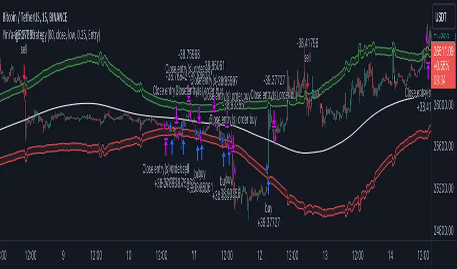
Strategy:Reversal-CatcherWhat
This is a plain and vanilla reversal based strategy for intraday (15m) timeframe on Futures prices of the assets.
Now what all it comprises of?
It finds out the dynamic support & resistance from Bollinger Band (20 period, 1.5 std dev).
It finds out the potential divergence of price deviation from 5 period exponential moving average (EMA).
If the previous candle (N-1) shows a divergence it confirms the reversal by checking the present candle (N) to be closed inside the Bollinger Band.
It confirms the momentum by checking RSI shows a crossover/crossunder to oversold (30) / overbought (70) region.
It also confirms whether the trend is up (then only reversal trade to short) or down (then only reversal trade to long). The trend is checked with EMA-21 and EMA-50.
Re-affirmation Condition : It re-affirms the position of two successive candles called as `hhLLong` and `hhLLShort` in the script.
Why
In Indian context, retail participants are pre-dominantly (yes- 80% of Indian daily volume) Options buyers mainly in weekly indices (Nifty, BankNifty, FinNifty, CNXMidcap, Sensex, Bankx .. well everyday is expiry now in India, except -- Thank God -- Saturday & Sunday).
And in Index Options the momentum plays a big role.
If one can catch a good reversal point the potential of high Risk-to-Reward trade (hence earn handsomely) is very likely (please note: there is no holy grail in trading. Nothing works 100%).
So this is the attempt to catch a reversal.
Re-affirmation of Reversal
hhLLong : It's a reversal point after an uptrend. It checks the relative positioning of current candle compared to that of previous candle. [The details are in the script. Check for variable hhLLong in script.
hhLLShort : It's a reversal point after a downtrend. It checks the relative positioning of current candle compared to that of previous candle. [The details are in the script. Check for variable hhLLShort in script.
Unique-ness
What's unique in it? Why we decided to publicly share this:
Already given the context of The Great Indian Options Buyers community. It should be helpful to them, we believe.
It takes Very Less Number of Trades with High Accuracy . Please check the result in NSE:NIFTY1! in 15m timeframe. 71% accuracy with roughly a trade in a month.
There is no point giving brokers' the brokerages taking 10 trades a day and ending not-so-good EoD. Better lets take less trades with better result possibility. .
Mention
There are many people uses this variation of Bolling Band, 5EMA
Many people use RSI, trends and relative positioning of candles.
--> We are grateful to all of them. It's really difficult to mention everyone's name. But all people somehow influence the thought process. Thanks for all of them.
Statutory Disclaimer
There is no silver bullet / holy grail in trading. Nothing works 100% time. One has to be careful about the loss (s)he can bear in case of the trade goes against.
We, as the author of this script, is not responsible for any trading or position decision one is taken based on the outcome of this.
It is our sole discretion to change, add, delete the portion or withdraw the whole script without any prior notice or intimation.
In Indian Context : We are not SEBI registered, will never be SEBI registered.
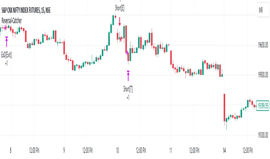
Nexus Blast Trading Strategy [Kaspricci]Nexus Blast Trading Strategy - Kaspricci
This indicator shows the different sessions during the day (London session, New York AM session, New York PM session and Asian session) by adding vertical lines and draws horizontal lines for the high and low during each session. Furthermore those lines turn red once the price has taken this high or low. Blue lines indicate liquidity not yet taken.
On top the indicator draws boxes of different color to indicate bullish and bearish Fair Value Gaps (FVG).
Happy to receive your feedback. Please leave a comment for bugs as well as ideas for improvement.
General Settings
Time Zone - used for marking sessions and end of day.
Sessions
Sessions - start and end time for each session based on set time zone
Number of Days back - for how many days in the past the startegy will draw strategy highs and lows. Theres is a maximum of 50 days defined.
FVG Settings
Threshold in Ticks - you can hide very small FVGs by increasing this threshold
FVG Colors - colors used for the bearish and bullish FVG box
This script is for educational purposes only! It is not meant to be a financial advice.
PS: The former strategy script was removed by TV, as it would violate several rules according to them.
Rolling Risk-Adjusted Performance RatiosThis simple indicator calculates and provides insights into different performance metrics of an asset - Sharpe, Sortino and Omega Ratios in particular. It allows users to customize the lookback period and select their preferred data source for evaluation of an asset.
Sharpe Ratio:
The Sharpe Ratio measures the risk-adjusted return of an asset by considering both the average return and the volatility or riskiness of the investment. A higher Sharpe Ratio indicates better risk-adjusted performance. It allows investors to compare different assets or portfolios and assess whether the returns adequately compensate for the associated risks. A higher Sharpe Ratio implies that the asset generates more return per unit of risk taken.
Sortino Ratio:
The Sortino Ratio is a variation of the Sharpe Ratio that focuses specifically on the downside risk or volatility of an asset. It takes into account only the negative deviations from the average return (downside deviation). By considering downside risk, the Sortino Ratio provides a more refined measure of risk-adjusted performance, particularly for investors who are more concerned with minimizing losses. A higher Sortino Ratio suggests that the asset has superior risk-adjusted returns when considering downside volatility.
Omega Ratio:
The Omega Ratio measures the probability-weighted ratio of gains to losses beyond a certain threshold or target return. It assesses the skewed nature of an asset's returns by differentiating between positive and negative returns and assigning more weight to extreme gains or losses. The Omega Ratio provides insights into the potential asymmetry of returns, highlighting the potential for significant positive or negative outliers. A higher Omega Ratio indicates a higher probability of achieving large positive returns compared to large negative returns.
Utility:
Performance Evaluation: Provides assessment of an asset's performance, considering both returns and risk factors.
Risk Comparison: Allows for comparing the risk-adjusted returns of different assets or portfolios. Helps identify investments with better risk-reward trade-offs.
Risk Management: Assists in managing risk exposure by evaluating downside risks and volatility.

NIFTY 50 5mint StrategyThis is an intraday strategy for NIFTY50 Based First candle High and Low breakout.
The strategy takes user inputs for the start and end dates, start and end months, and start and end years, which define the time range to trade. The user can also specify the maximum number of trades to take during the time range and the length of the Exponential Moving Average ( EMA ) used in the strategy
In this strategy, the First candle's high and low are calculated and used as entry and exit points for trades. If the close price breaks above the First candle's high, a buy signal is generated. Conversely, if the close price breaks below the First candle's low, a sell signal is generated.
The strategy uses the Exponential Moving Average ( EMA ) as a filter to close entered positions either long or short, EMA also acts Target. If the close price falls below the EMA, a long position is closed, and if the close price rises above the EMA, a short position is closed or the PreviousCandleClose is above the First candle's high a short position is closed, When the PreviousCandleClose is below the First candle's low a long position is closed, First candle's high act as Stoploss
The strategy limits the number of trades taken within the specified time range, and if the time range is exceeded, all positions are closed.
Finally, the strategy plots the First candle's high and low, EMAs on the chart for visual reference.
Default settings work best with the 5mint candle, you may tweak settings according to your needs.
backtesting helps in interpreting how the trading strategy would have behaved in the past, and forward testing (paper trading) informs the traders how it would perform now.

Trend & atr day & calcHi!
Why for what and how in this script?
At the time of publication the script consists of three modules, it may increase in the future.
1. Bottom left corner : daytime ATR module
(idea and basis of the author's script - ???)
- The size of the daily ATR based on 14 bars;
- intraday ATR progress;
- colour indication of the progress status, for easier visual perception (green < 70%, yellow 70-90 and red over 90% of ATR)
By evaluating the progress of the daily ATR, it is possible to suggest and expedient to enter/exit/hold a trade.
2. Top right: trend module
The trend is calculated based on Bill Williams' alligator indicator
- trend status on specified timeframes for the current ticker;
- colour indication for visual perception (green - growing trend, yellow - alligator is sleeping, red - downtrend)
Do not forget that the alligator is based on moving averages with the resulting consequences.
Its purpose is to assess the state of the trend on other ticker TFs, without additional actions (switching to another screen or TF)
3. In the bottom left corner - risk and position calculator
(based on an idea of the risk calculator by @andrei.bunulu)
It helps to determine the advisability of entering the trade and also what size position to enter into the trade, within money management strategy chosen.
- The calculator works in two directions: long deal and short deal (short deal calculation is enabled by check-box in settings)
- two calculation methods:
a. based on the set stop loss % (default is 0.3%), in this mode the stop and takeout level is automatically calculated (default is 1 / 3).
b. by entering the desired price levels (entry, stop and take profit points)
To make this work correctly please do not forget to choose the type of calculation (% or price) in the settings, and the currency symbol (for visual representation in the results).
The calculator can take into account the set commissions and spreads.
When hovering over the module - tooltips are displayed.
Each module can be enabled / disabled in the settings.
The size and arrangement of the modules is made for joint use with the script - "Abnormal Bar".
/// а по-русски это так ///
Привет!
Зачем для чего и как в этом скрипте?
На момент публикации скрипт состоит из трех модулей, возможно в будущем увеличится.
1. В левом нижнем углу : модуль дневного ATR
(идея и основа скрипт автора - ???)
- размер дневной ATR на основании 14 баров;
- прогресс ATR внутри дня;
- цветовая индикация состояния прогресса, для более простого визуального восприятия (зеленый < 70%, желтый 70-90 и красный более 90% ATR)
Оценивая прогресс дневного ATR, можно предположить и целесообразности входа / выхода / удержания из сделки.
2. В правом верхнем углу: модуль тренда
Тренд рассчитывается на основе индикатора - аллигатор Билла Вильямса
- состояние тренда на указанных таймфреймах для текущего тикера;
- цветовая индикация для визуального восприятия (зеленый - растущий тренд, желтый - аллигатор спит, красный - нисходящий тренд)
Не забываем, что аллигатор построен на основе скользящих средних с вытекающими последствиями.
Назначение - оценить состояние тренда на других ТФ тикера, без дополнительных действий (переключения на другой экран или ТФ)
3. В нижнем левом углу - калькулятор рисков и позиции
(на основе идеи калькулятора аuthor: @andrei.bunulu)
Помогает определить целесообразность входа в сделку, а также каким размером позиции входить в сделку, в рамках выбранной стратегии мани менеджмента.
- калькулятор работает в два направления: длинная и короткая сделка (расчет по короткой включается в настройках чек-боксом)
- два варианта расчета:
а. на основании установленного % стоп лосса (по-умолчанию 0,3%), при этом режиме происходит автоматический расчет уровня стопа и тейка (по умолчанию 1 / 3).
b. путем ввода данных желаемых уровней цены (точки входа, стопа и тейк профита)
Для корректной работы не забываем в настройках выбирать тип расчета (% или цена), а также символ валюты (для визуального отображения в итогах).
Калькулятор может учитывать установленный размер комиссий и спреда.
При наведении на модуль - отображаются подсказки.
Каждый модуль можно включить / выключить в настройках.
Размер и расположение модулей сделано для совместного использования со скриптом - "Abnormal Bar"

Physics CandlesPhysics Candles embed volume and motion physics directly onto price candles or market internals according to the cyclic pattern of financial securities. The indicator works on both real-time “ticks” and historical data using statistical modeling to highlight when these values, like volume or momentum, is unusual or relatively high for some periodic window in time. Each candle is made out of one or more sub-candles that each contain their own information of motion, which converts to the color and transparency, or brightness, of that particular candle segment. The segments extend throughout the entire candle, both body and wicks, and Thick Wicks can be implemented to see the color coding better. This candle segmentation allows you to see if all the volume or energy is evenly distributed throughout the candle or highly contained in one small portion of it, and how intense these values are compared to similar time periods without going to lower time frames. Candle segmentation can also change a trader’s perspective on how valuable the information is. A “low” volume candle, for instance, could signify high value short-term stopping volume if the volume is all concentrated in one segment.
The Candles are flexible. The physics information embedded on the candles need not be from the same price security or market internal as the chart when using the Physics Source option, and multiple Candles can be overlayed together. You could embed stock price Candles with market volume, market price Candles with stock momentum, market structure with internal acceleration, stock price with stock force, etc. My particular use case is scalping the SPX futures market (ES), whose price action is also dictated by the volume action in the associated cash market, or SPY, as well as a host of other securities. Physics allows you to embed the ES volume on the SPY price action, or the SPY volume on the ES price action, or you can combine them both by overlaying two Candle streams and increasing the Number of Overlays option to two. That option decreases the transparency levels of your coloring scheme so that overlaying multiple Candles converges toward the same visual color intensity as if you had one. The Candle and Physics Sources allows for both Symbols and Spreads to visualize Candle physics from a single ticker or some mathematical transformation of tickers.
Due to certain TradingView programming restrictions, each Candle can only be made out of a maximum of 8 candle segments, or an “8-bit” resolution. Since limits are just an opportunity to go beyond, the user has the option to stack multiple Candle indicators together to further increase the candle resolution. If you don’t want to see the Candles for some particular period of the day, you can hide them, or use the hiding feature to have multiple Candles calibrated to show multiple parts of the trading day. Securities tend to have low volume after hours with sharp spikes at the open or close. Multiple Candles can be used for multiple parts of the trading day to accommodate these different cycles in volume.
The Candles do not need be associated with the nominal security listed on the TV chart. The Candle Source allows the user to look at AAPL Candles, for instance, while on a TSLA or SPY chart, each with their respective volume actions integrated into the candles, for instance, to allow the user to see multiple security price and volume correlation on a single chart.
The physics information currently embeddable on Candles are volume or time, velocity, momentum, acceleration, force, and kinetic energy. In order to apply equations of motion containing a mass variable to financial securities, some analogous value for mass must be assumed. Traders often regard volume or time as inextricable variables to a securities price that can indicate the direction and strength of a move. Since mass is the inextricable variable to calculating the momentum, force, or kinetic energy of motion, the user has the option to assume either time or volume is analogous to mass. Volume may be a better option for mass as it is not strictly dependent on the speed of a security, whereas time is.
Data transformations and outlier statistics are used to color code the intensity of the physics for each candle segment relative to past periodic behavior. A million shares during pre-market or a million shares during noontime may be more intense signals than a typical million shares traded at the open, and should have more intense color signals. To account for a specific cyclic behavior in the market, the user can specify the Window and Cycle Time Frames. The Window Time Frame splits up a Cycle into windows, samples and aggregates the statistics for each window, then compares the current physics values against past values in the same window. Intraday traders may benefit from using a Daily Cycle with a 30-minute Window Time Frame and 1-minute Sample Time Frame. These settings sample and compare the physics of 1-minute candles within the current 30-minute window to the same 30-minute window statistics for all past trading days, up until the data limit imposed by TradingView, or until the Data Collection Start Date specified in the settings. Longer-term traders may benefit from using a Monthly Cycle with a Weekly Time Frame, or a Yearly Cycle with a Quarterly Time Frame.
Multiple statistics and data transformation methods are available to convey relative intensity in different ways for different trading signals. Physics Candles allows for both Normal and Log-Normal assumptions in the physics distribution. The data can then be transformed by Linear, Logarithmic, Z-Score, or Power-Law scoring, where scoring simply assigns an intensity to the relative physics value of each candle segment based on some mathematical transformation. Z-scoring often renders adequate detection by scoring the segment value, such as volume or momentum, according to the mean and standard deviation of the data set in each window of the cycle. Logarithmic or power-law transformation with a gamma below 1 decreases the disparity between intensities so more less-important signals will show up, whereas the power-law transformation with gamma values above 1 increases the disparity between intensities, so less more-important signals will show up. These scores are then converted to color and transparency between the Min Score and the Max Score Cutoffs. The Auto-Normalization feature can automatically pick these cutoffs specific to each window based on the mean and standard deviation of the data set, or the user can manually set them. Physics was developed with novices in mind so that most users could calibrate their own settings by plotting the candle segment distributions directly on the chart and fiddling with the settings to see how different cutoffs capture different portions of the distribution and affect the relative color intensities differently. Security distributions are often skewed with fat-tails, known as kurtosis, where high-volume segments for example, have a higher-probabilities than expected for a normal distribution. These distribution are really log-normal, so that taking the logarithm leads to a standard bell-shaped distribution. Taking the Z-score of the Log-Normal distribution could make the most statistical sense, but color sensitivity is a discretionary preference.
Background Philosophy
This indicator was developed to study and trade the physics of motion in financial securities from a visually intuitive perspective. Newton’s laws of motion are loosely applied to financial motion:
“A body remains at rest, or in motion at a constant speed in a straight line, unless acted upon by a force”.
Financial securities remain at rest, or in motion at constant speed up or down, unless acted upon by the force of traders exchanging securities.
“When a body is acted upon by a force, the time rate of change of its momentum equals the force”.
Momentum is the product of mass and velocity, and force is the product of mass and acceleration. Traders render force on the security through the mass of their trading activity and the acceleration of price movement.
“If two bodies exert forces on each other, these forces have the same magnitude but opposite directions.”
Force arises from the interaction of traders, buyers and sellers. One body of motion, traders’ capitalization, exerts an equal and opposite force on another body of motion, the financial security. A securities movement arises at the expense of a buyer or seller’s capitalization.
Volume
The premise of this indicator assumes that volume, v, is an analogous means of measuring physical mass, m. This premise allows the application of the equations of motion to the movement of financial securities. We know from E=mc^2 that mass has energy. Energy can be used to create motion as kinetic energy. Taking a simple hypothetical example, the interaction of one short seller looking to cover lower and one buyer looking to sell higher exchange shares in a security at an agreed upon price to create volume or mass, and therefore, potential energy. Eventually the short seller will actively cover and buy the security from the previous buyer, moving the security higher, or the buyer will actively sell to the short seller, moving the security lower. The potential energy inherent in the initial consolidation or trading activity between buy and seller is now converted to kinetic energy on the subsequent trading activity that moves the securities price. The more potential energy that is created in the consolidation, the more kinetic energy there is to move price. This is why point and figure traders are said to give price targets based on the level of volatility or size of a consolidation range, or why Gann traders square price and time, as time is roughly proportional to mass and trading activity. The build-up of potential energy between short sellers and buyers in GME or TSLA led to their explosive moves beyond their standard fundamental valuations.
Position
Position, p, is simply the price or value of a financial security or market internal.
Time
Time, t, is another means of measuring mass to discover price behavior beyond the time snapshots that simple candle charts provide. We know from E=mc^2 that time is related to rest mass and energy given the speed of light, c, where time ≈ distance * sqrt(mass/E). This relation can also be derived from F=ma. The more mass there is, the longer it takes to compute the physics of a system. The more energy there is, the shorter it takes to compute the physics of a system. Similarly, more time is required to build a “resting” low-volatility trading consolidation with more mass. More energy added to that trading consolidation by competing buyers and sellers decreases the time it takes to build that same mass. Time is also related to price through velocity.
Velocity = (p(t1) – p(t0)) / p(t0)
Velocity, v, is the relative percent change of a securities price, p, over a period of time, t0 to t1. The period of time is between subsequent candles, and since time is constant between candles within the same timeframe, it is not used to calculate velocity or acceleration. Price moves faster with higher velocity, and slower with slower velocity, over the same fixed period of time. The product of velocity and mass gives momentum.
Momentum = mv
This indicator uses physics definition of momentum, not finance’s. In finance, momentum is defined as the amount of change in a securities price, either relative or absolute. This is definition is unfortunate, pun intended, since a one dollar move in a security from a thousand shares traded between a few traders has the exact same “momentum” as a one dollar move from millions of shares traded between hundreds of traders with everything else equal. If momentum is related to the energy of the move, momentum should consider both the level of activity in a price move, and the amount of that price move. If we equate mass to volume to account for the level of trading activity and use physics definition of momentum as the product of mass and velocity, this revised definition now gives a thousand-times more momentum to a one-dollar price move that has a thousand-times more volume behind it. If you want to use finance’s volume-less definition of momentum, use velocity in this indicator.
Acceleration = v(t1) – v(t0)
Acceleration, a, is the difference between velocities over some period of time, t0 to t1. Positive acceleration is necessary to increase a securities speed in the positive direction, while negative acceleration is necessary to decrease it. Acceleration is related to force by mass.
Force = ma
Force is required to change the speed of a securities valuation. Price movements with considerable force have considerably more impact on future direction. A change in direction requires force.
Kinetic Energy = 0.5mv^2
Kinetic energy is the energy that a financial security gains from the change in its velocity by force. The built-up of potential energy in trading consolidations can be converted to kinetic energy on a breakout from the consolidation.
Cycle Theory and Relativity
Just as the physics of motion is relative to a point of reference, so too should the physics of financial securities be relative to a point of reference. An object moving at a 100 mph towards another object moving in the same direction at 100 mph will not appear to be moving relative to each other, nor will they collide, but from an outsider observer, the objects are going 100 mph and will collide with significant impact if they run into a stationary object relative to the observer. Similarly, trading with a hundred thousand shares at the open when the average volume is a couple million may have a much smaller impact on the price compared to trading a hundred thousand shares pre-market when the average volume is ten thousand shares. The point of reference used in this indicator is the average statistics collected for a given Window Time Frame for every Cycle Time Frame. The physics values are normalized relative to these statistics.
Examples
The main chart of this publication shows the Force Candles for the SPY. An intense force candle is observed pre-market that implicates the directional overtone of the day. The assumption that direction should follow force arises from physical observation. If a large object is accelerating intensely in a particular direction, it may be fair to assume that the object continues its direction for the time being unless acted upon by another force.
The second example shows a similar Force Candle for the SPY that counters the assumption made in the first example and emphasizes the importance of both motion and context. While it’s fair to assume that a heavy highly accelerating object should continue its course, if that object runs into an obstacle, say a brick wall, it’s course may deviate. This example shows SPY running into the 50% retracement wall from the low of Mar 2020, a significant support level noted in literature. The example also conveys Gann’s idea of “lost motion”, where the SPY penetrated the 50% price but did not break through it. A brick wall is not one atom thick and price support is not one tick thick. An object can penetrate only one layer of a wall and not go through it.
The third example shows how Volume Candles can be used to identify scalping opportunities on the SPY and conveys why price behavior is as important as motion and context. It doesn’t take a brick wall to impede direction if you know that the person driving the car tends to forget to feed the cats before they leave. In the chart below, the SPY breaks down to a confluence of the 5-day SMA, 20-day SMA, and an important daily trendline (not shown) after the bullish bounce from the 50% retracement days earlier. High volume candles on the SMA signify stopping volume that reverse price direction. The character of the day changes. Bulls become more aggressive than bears with higher volume on upswings and resistance, whiles bears take on a defensive position with lower volume on downswings and support. High volume stopping candles are seen after rallies, and can tell you when to take profit, get out of a position, or go short. The character change can indicate that its relatively safe to re-enter bullish positions on many major supports, especially given the overarching bullish theme from the large reaction off the 50% retracement level.
The last example emphasizes the importance of relativity. The Volume Candles in the chart below are brightest pre-market even though the open has much higher volume since the pre-market activity is much higher compared to past pre-markets than the open is compared to past opens. Pre-market behavior is a good indicator for the character of the day. These bullish Volume Candles are some of the brightest seen since the bounce off the 50% retracement and indicates that bulls are making a relatively greater attempt to bring the SPY higher at the start of the day.
Infrequently Asked Questions
Where do I start?
The default settings are what I use to scalp the SPY throughout most of the extended trading day, on a one-minute chart using SPY volume. I also overlay another Candle set containing ES future volume on the SPY price structure by setting the Physics Source to ES1! and the Number of Overlays setting to 2 for each Candle stream in order to account for pre- and post-market trading activity better. Since the closing volume is exponential-like up until the end of the regular trading day, adding additional Candle streams with a tighter Window Time Frame (e.g., 2-5 minute) in the last 15 minutes of trading can be beneficial. The Hide feature can allow you to set certain intraday timeframes to hide one Candle set in order to show another Candle set during that time.
How crazy can you get with this indicator?
I hope you can answer this question better. One interesting use case is embedding the velocity of market volume onto an internal market structure. The PCTABOVEVWAP.US is a market statistic that indicates the percent of securities above their VWAP among US stocks and is helpful for determining short term trends in the US market. When securities are rising above their VWAP, the average long is up on the day and a rising PCTABOVEVWAP.US can be viewed as more bullish. When securities are falling below their VWAP, the average short is up on the day and a falling PCTABOVEVWAP.US can be viewed as more bearish. (UPVOL.US - DNVOL.US) / TVOL.US is a “spread” symbol, in TV parlance, that indicates the decimal percent difference between advancing volume and declining volume in the US market, showing the relative flow of volume between stocks that are up on the day, and stocks that are down on the day. Setting PCTABOVEVWAP.US in the Candle Source, (UPVOL.US - DNVOL.US) / TVOL.US in the Physics Source, and selecting the Physics to Velocity will embed the relative velocity of the spread symbol onto the PCTABOVEVWAP.US candles. This can be helpful in seeing short term trends in the US market that have an increasing amount of volume behind them compared to other trends. The chart below shows Volume Candles (top) and these Spread Candles (bottom). The first top at 9:30 and second top at 10:30, the high of the day, break down when the spread candles light up, showing a high velocity volume transfer from up stocks to down stocks.
How do I plot the indicator distribution and why should I even care?
The distribution is visually helpful in seeing how different normalization settings effect the distribution of candle segments. It is also helpful in seeing what physics intensities you want to ignore or show by segmenting part of the distribution within the Min and Max Cutoff values. The intensity of color is proportional to the physics value between the Min and Max Cutoff values, which correspond to the Min and Max Colors in your color scheme. Any physics value outside these Min and Max Cutoffs will be the same as the Min and Max Colors.
Select the Print Windows feature to show the window numbers according to the Cycle Time Frame and Window Time Frame settings. The window numbers are labeled at the start of each window and are candle width in size, so you may need to zoom into to see them. Selecting the Plot Window feature and input the window number of interest to shows the distribution of physics values for that particular window along with some statistics.
A log-normal volume distribution of segmented z-scores is shown below for 30-minute opening of the SPY. The Min and Max Cutoff at the top of the graph contain the part of the distribution whose intensities will be linearly color-coded between the Min and Max Colors of the color scheme. The part of the distribution below the Min Cutoff will be treated as lowest quality signals and set to the Min Color, while the few segments above the Max Cutoff will be treated as the highest quality signals and set to the Max Color.
What do I do if I don’t see anything?
Troubleshooting issues with this indicator can involve checking for error messages shown near the indicator name on the chart or using the Data Validation section to evaluate the statistics and normalization cutoffs. For example, if the Plot Window number is set to a window number that doesn’t exist, an error message will tell you and you won’t see any candles. You can use the Print Windows option to show windows that do exist for you current settings. The auto-normalization cutoff values may be inappropriate for your particular use case and literally cut the candles out of the chart. Try changing the chart time frame to see if they are appropriate for your cycle, sample and window time frames. If you get a “Timeframe passed to the request.security_lower_tf() function must be lower than the timeframe of the main chart” error, this means that the chart timeframe should be increased above the sample time frame. If you get a “Symbol resolve error”, ensure that you have correct symbol or spread in the Candle or Physics Source.
How do I see a relative physics values without cycles?
Set the Window Time Frame to be equal to the Cycle Time Frame. This will aggregate all the statistics into one bucket and show the physics values, such as volume, relative to all the past volumes that TV will allow.
How do I see candles without segmentation?
Segmentation can be very helpful in one context or annoying in another. Segmentation can be removed by setting the candle resolution value to 1.
Notes
I have yet to find a trading platform that consistently provides accurate real-time volume and pricing information, lacking adequate end-user data validation or quality control. I can provide plenty of examples of real-time volume counts or prices provided by TradingView and other platforms that were significantly off from what they should have been when comparing against the exchanges own data, and later retroactively corrected or not corrected at all. Since no indicator can work accurately with inaccurate data, please use at your own discretion.
The first version is a beta version. Debugging and validating code in Pine script is difficult without proper unit testing. Please report any bugs with enough information to reproduce them and indicate why they are important. I also encourage you to export the data from TradingView and verify the calculations for your particular use case.
The indicator works on real-time updates that occur at a higher frequency than the candle time frame, which TV incorrectly refers to as ticks. They use this terminology inaccurately as updates are really aggregated tick data that can take place at different prices and may not accurately reflect the real tick price action. Consequently, this inaccuracy also impacts the real-time segmentation accuracy to some degree. TV does not provide a means of retaining “tick” information, so the higher granularity of information seen real-time will be lost on a disconnect.
TV does not provide time and sales information. The volume and price information collected using the Sample Time Frame is intraday, which provides only part of the picture. Intraday volume is generally 50 to 80% of the end of day volume. Consequently, the daily+ OHLC prices are intraday, and may differ significantly from exchanged settled OHLC prices.
The Cycle and Window Time Frames refer to calendar days and time, not trading days or time. For example, the first window week of a monthly cycle is the first seven days of the month, not the first Monday through Friday of trading for the month.
Chart Time Frames that are higher than the Window Time Frames average the normalized physics for price action that occurred within a given Candle segment. It does not average price action that did not occur.
One of the main performance bottleneck in TradingView’s Pine Script is client-side drawing and plotting. The performance of this indicator can be increased by lowering the resolution (the number of sub-candles this indicator plots), getting a faster computer, or increasing the performance of your computer like plugging your laptop in and eliminating unnecessary processes.
The statistical integrity of this indicator relies on the number of samples collected per sample window in a given cycle. Higher sample counts can be obtained by increasing the chart time frame or upgrading the TradingView plan for a higher bar count. While increasing the chart time frame doesn’t increase the visual number of bars plotted on the chart, it does increase the number of bars that can be pulled at a lower time frame, up to 100,000.
Due to a limitation in Pine Scripts request_lower_tf() function, using a spread symbol will only work for regular trading hours, not extended trading hours.
Ideally, velocity or momentum should be calculated between candle closes. To eliminate the need to deal with price gaps that would lead to an incorrect statistical distributions, momentum is calculated between candle open and closes as a percent change of the price or value, which should not be an issue for most liquid securities.