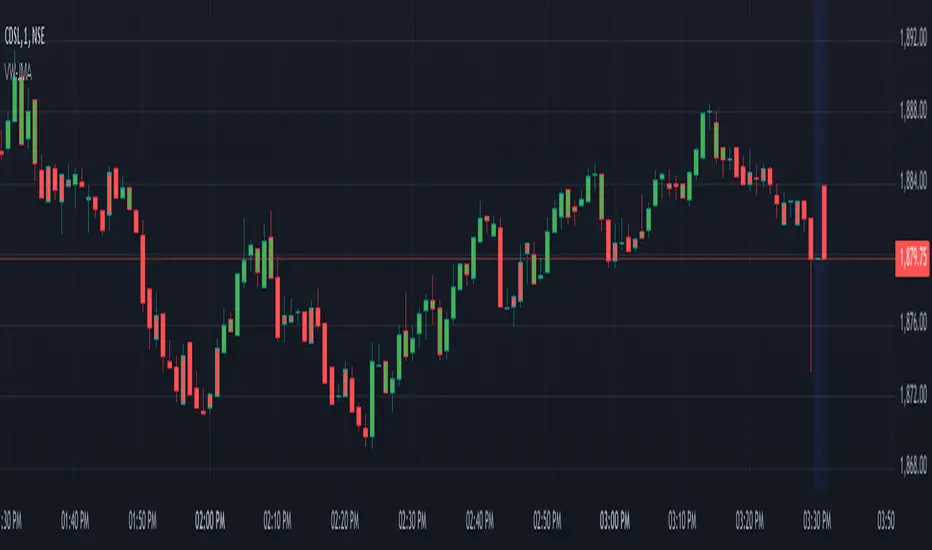
Volume Weighted Jurik Moving AverageThe Jurik Moving Average (JMA) is a smoothing indicator that is designed to improve upon traditional moving averages by reducing lag while enhancing responsiveness to price movements. It was created by Jurik Research and is often used to track trends with greater accuracy and minimal delay. The JMA is based on a combination of **exponential smoothing** and **phase adjustments**, making it more adaptable to varying market conditions compared to standard moving averages like SMA (Simple Moving Average) or EMA (Exponential Moving Average).
The core advantage of the JMA lies in its ability to adjust to price changes without excessively lagging, which is a common issue with traditional moving averages. It incorporates a **phase parameter** that can be adjusted to smooth out the signal further or make it more responsive to recent price action. This phase adjustment allows traders to fine-tune the JMA's sensitivity to the market, optimizing it for different timeframes and trading strategies.
How JMA Works and Benefits of Adding Volume Weight
The JMA works by applying a **smoothing process** to price data while allowing for adjustments through its phase and power parameters. These parameters help control the degree of smoothness and responsiveness. The result is a curve that follows price trends closely but with less lag than traditional moving averages.
Adding **volume weighting** to the JMA enhances its ability to reflect market activity more accurately. Just like the **Volume-Weighted Moving Average (VWMA)**, volume-weighting adjusts the moving average based on the strength of trading volume, meaning that price movements with higher volume will have a greater influence on the JMA. This can help traders identify trends that are supported by significant market participation, making the moving average more reliable.
The benefit of a volume-weighted JMA is that it responds more effectively to price movements that occur during periods of high trading volume, which are often considered more significant. This can help traders avoid false signals that may occur during low-volume periods when price changes may not reflect true market sentiment. By incorporating volume into the calculation, the JMA becomes more aligned with real market conditions, enhancing its effectiveness for trend identification and decision-making.
Tìm kiếm tập lệnh với "moving averages"
Magnificent 7 Overall Percentage Change with MA and Angle LabelsMagnificent 7 Overall Percentage Change with MA and Angle Labels
Overview:
The "Magnificent 7 Overall Percentage Change with MA and Angle Labels" indicator tracks the percentage change of seven key tech stocks (Apple, Microsoft, Amazon, NVIDIA, Tesla, Meta, and Alphabet) and displays their overall average percentage change on the chart. It also provides a moving average of this overall change and calculates the angle of the moving average to help traders gauge the momentum and direction of the overall trend.
How it works:
Real-Time Percentage Change: The indicator calculates the percentage change of each of the "Magnificent 7" stocks compared to their previous day's closing price, giving a snapshot of the market's performance.
Overall Average: It then computes the average of the seven stocks' percentage changes to reflect the broader movement of these major tech companies.
Moving Average: The indicator offers a choice of four types of moving averages (SMA, EMA, WMA, or VWMA) to smooth the overall percentage change, allowing traders to focus on the trend rather than short-term fluctuations.
Slope and Angle Calculation: To provide additional insights, the indicator calculates the slope of the moving average and converts it into an angle (in degrees). This can help traders determine the strength of the trend—steeper angles often indicate stronger momentum.
Key Features:
Percentage Change of the "Magnificent 7":
Tracks the percentage change of Apple (AAPL), Microsoft (MSFT), Amazon (AMZN), NVIDIA (NVDA), Tesla (TSLA), Meta (META), and Alphabet (GOOGL) on the current chart's timeframe.
Overall Average Change:
Computes the average percentage change across all seven stocks, giving a combined view of how the most influential tech stocks are performing.
Customizable Moving Averages:
Offers four types of moving averages (SMA, EMA, WMA, VWMA) to provide flexibility in tracking the trend of the overall percentage change.
Angle Calculation:
Measures the angle of the moving average in degrees, which helps assess the strength of the market’s momentum. Alerts and visual cues can be triggered based on the angle's steepness.
Visual Cues:
The percentage change is plotted in green when positive and red when negative, with a background color that changes accordingly. A zero line is plotted for reference.
Use Case:
This indicator is ideal for traders and investors looking to track the collective performance of the most dominant tech companies in the market. It provides real-time insights into how the "Magnificent 7" stocks are moving together and offers clues about potential market momentum based on the direction and angle of their average percentage change.
Customization:
Moving Average Type and Length: Choose between different types of moving averages (SMA, EMA, WMA, VWMA) and adjust the length to suit your preferred timeframe.
Angle Threshold: Set an angle threshold to trigger alerts when the moving average slope becomes too steep, indicating strong momentum.
Alerts:
Alerts can be created based on the crossing of the moving average or when the angle of the moving average exceeds a specified threshold. This ensures traders are notified when the trend is accelerating or decelerating significantly.
Conclusion:
The "Magnificent 7 Overall Percentage Change with MA and Angle Labels" indicator is a powerful tool for those wanting to monitor the performance of the most influential tech stocks, analyze their overall trend, and receive timely alerts when market conditions shift.

TechniTrend: Average VolatilityTechniTrend: Average Volatility
Description:
The "Average Volatility" indicator provides a comprehensive measure of market volatility by offering three different types of volatility calculations: High to Low, Body, and Shadows. The indicator allows users to apply various types of moving averages (SMA, EMA, SMMA, WMA, and VWMA) on these volatility measures, enabling a more flexible approach to trend analysis and volatility tracking.
Key Features:
Customizable Volatility Types:
High to Low: Measures the range between the highest and lowest prices in the selected period.
Body: Measures the absolute difference between the opening and closing prices of each candle (just the body of the candle).
Shadows: Measures the difference between the wicks (shadows) of the candle.
Flexible Moving Averages:
Choose from five different types of moving averages to apply on the calculated volatility:
SMA (Simple Moving Average)
EMA (Exponential Moving Average)
SMMA (RMA) (Smoothed Moving Average)
WMA (Weighted Moving Average)
VWMA (Volume-Weighted Moving Average)
Custom Length:
Users can customize the period length for the moving averages through the Length input.
Visualization:
Three separate plots are displayed, each representing the average volatility of a different type:
Blue: High to Low volatility.
Green: Candle body volatility.
Red: Candle shadows volatility.
-------------------------------------------
This indicator offers a versatile and highly customizable tool for analyzing volatility across different components of price movement, and it can be adapted to different trading styles or market conditions.

Atareum Volume Ichimuku CandleAVIC (Atareum Volume Ichimoku Candles) is clearly an awesome indicator that is based on Ichimoku concepts by combination with volume. This is a new approach of volume candles that is combined with Ichimoku concepts and creates such a powerful tool to trace the market and assists traders to make better decisions, truly.
Concept:
Using Ichimoku leading periods and calculations on redesigning new candles in combination with volume, that makes unique reform candles on Tenkansen movement, but these new candles clearly omit noises in combination with volume, and then the new redesigned system of cloud calculations builds, new series of data for Senko Span A and Senko Span B which is so odd in first view, because they will barely ever cross each other, but they show very more informative and useful.
Parameters:
Section 1 : Candle colour setting for flourishing just as you desire !
Section 2 : Defining Periods of standard Ichimoku and source of candle data in combination with determining the smoothing type of moving averages and signal period.
Section 3 : Select using Heikin Ashi based candles alongside with redesigned cloud calculation type and three additional moving averages which can plot on each newly generated candles and standard candles on a chart with the type mode defined in the previous section.
Note: if you want to omit any or all of these moving averages, you can use 0 in period, instead of selecting "None" in the plot moving option!
Usage :
Overall:
Regardless of the additional moving averages which will lead to so many situations of market according to their types and designs, that is four different period for new redesign AVIC and three period for standard chart. You can easily select periods and type for these moving averages. Also, do not forget that signal moving averages is shown only on AVIC chart and have two different colour for upward and downward trends. Other moving averages are plot by just one single colour.
Cloud levels are so important because AVIC candles show respect to them and when they break the clouds upward or downward it's surly beginning of a trend that is may last long. Also when cloud levels flatten, it is determining a support or resistance according to up cloud or down cloud nature and as long as they will continue or repeated periodically on same level of AVIC chart, it will implement their weakness or strength.
Support and Resistance:
Any flattens of cloud up or down level means the support or resistance level due to its nature, but important thing is how long the cloud lasts flatten or how many times repeated in the same level in AVIC chart.
For plotting the support or resistance you should trace first candle of start of flattens in standard chart just like following picture.
Divergence:
All Higher high or Lower low of standard chart has its reflect in AVIC chart but there is secret in it, It is named divergence. When standard chart price candles generating lower low but the AVIC chart candles do not cross the bottom, it means we will spike high as soon as AVIC candle chart complete its divergence. You can see perfect example in following picture.
Cloud level Ends
When cloud down level become flattens and cloud up level start a bull run it means we will face a great up trend movement but as soon as cloud down level starts to move up it mean we are going to finish the bull run and maybe it goes with consolidation phase or reversal phase. This reaction is exactly happen in vice versa for bear run trend. You can see both examples in following pictures.
Note: if we face end of bull run and cloud down level make a U turn shape upside down it means we will have reversal phase even not too long but it is sharp and fast reversal. If cloud down level just turn right slightly, it means we should have consolidation phase, mostly or we can continue the last trend slightly. All these situations can happen in vice versa bear run. You can see example in following picture.
Signals:
Long but risky:
You can go long when AVIC candles are green and be in position as long as they are not change in colour.
Long and safe :
You can go long when AVIC candles cross up cloud down level and be in position as long as AVIC candles cross down cloud up level.
Long and sure:
You can go long when AVIC candles cross up cloud up level and be in position as long as AVIC candles cross down cloud down level.
Short but risky:
You can go short when AVIC candles are red and be in position as long as they are not change in colour.
Short and safe :
You can go short when AVIC candles cross down cloud up level and be in position as long as AVIC candles cross up cloud down level.
Short and sure:
You can go short when AVIC candles cross down cloud down level and be in position as long as AVIC candles cross up cloud up level.
Notice : Candles with large body are so strong but if a body candle is weak or flatten it may a signal of changing colour and direction, especially when using Heikin Ashi type.
It is the result of many years of experience in markets and there are so many details about this AVIC chart which I am in the experiment phase to publish in the future, so please help me with your ideas and do not hesitate to comment and inform me any suggestions or criticism.

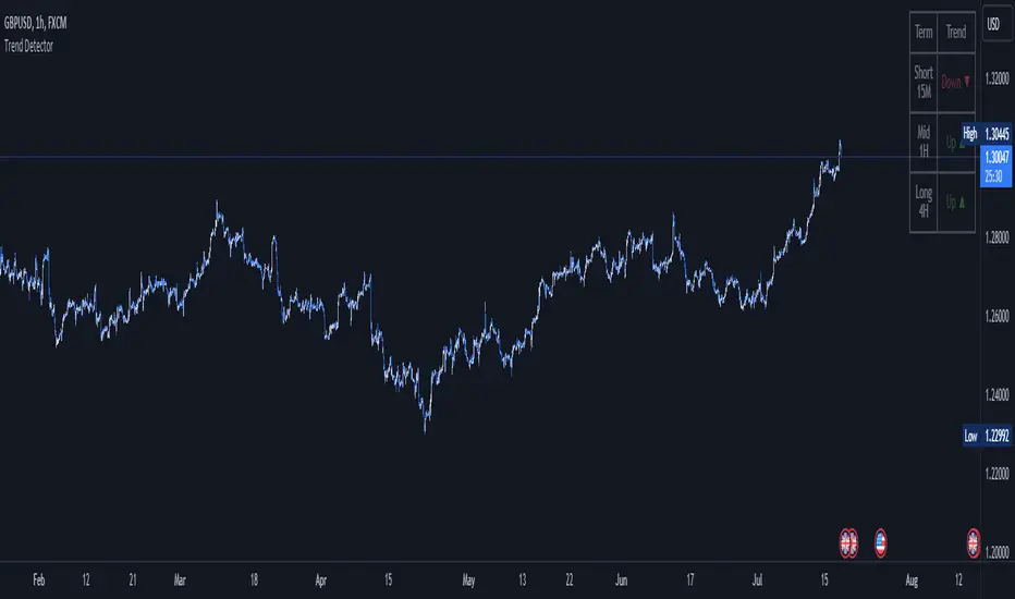
Trend DetectorThe Trend Detector indicator is a powerful tool to help traders identify and visualize market trends with ease. This indicator uses multiple moving averages (MAs) of different timeframes to provide a comprehensive view of market trends, making it suitable for traders of all experience levels.
█ USAGE
This indicator will automatically plot the chosen moving averages (MAs) on your chart, allowing you to visually assess the trend direction. Additionally, a table displaying the trend data for each selected MA timeframe is included to provide a quick overview.
█ FEATURES
1. Customizable Moving Averages: The indicator supports various types of moving averages, including Simple (SMA) , Exponential (EMA) , Smoothed (RMA) , Weighted (WMA) , and Volume-Weighted (VWMA) . You can select the type and length for each MA.
2. Multiple Timeframes: Plot moving averages for different timeframes on a single chart, including fast (short-term) , mid (medium-term) , and slow (long-term) MAs.
3. Trend Detector Table: A customizable table displays the trend direction (Up or Down) for each selected MA timeframe, providing a quick and easy way to assess the market's overall trend.
4. Customizable Appearance: Adjust the colors, frame, border, and text of the Trend Detector Table to match your chart's style and preferences.
5. Wait for Timeframe Close: Option to wait until the selected timeframe closes to plot the MA, which will remove the gaps.
█ CONCLUSION
The Trend Detector indicator is a versatile and user-friendly tool designed to enhance your trading strategy. By providing a clear visualization of market trends across multiple timeframes, this indicator helps you make informed trading decisions with confidence and trade with the market trend. Whether you're a day trader or a long-term investor, this indicator is an essential addition to your trading toolkit.
█ IMPORTANT
This indicator is a tool to aid in your analysis and should not be used as the sole basis for trading decisions. It is recommended to use this indicator in conjunction with other tools and perform comprehensive market analysis before making any trades.
Happy trading!
Leading T3Hello Fellas,
Here, I applied a special technique of John F. Ehlers to make lagging indicators leading. The T3 itself is usually not realling the classic lagging indicator, so it is not really needed, but I still publish this indicator to demonstrate this technique of Ehlers applied on a simple indicator.
The indicator does not repaint.
In the following picture you can see a comparison of normal T3 (purple) compared to a 2-bar "leading" T3 (gradient):
The range of the gradient is:
Bottom Value: the lowest slope of the last 100 bars -> green
Top Value: the highest slope of the last 100 bars -> purple
Ehlers Special Technique
John Ehlers did develop methods to make lagging indicators leading or predictive. One of these methods is the Predictive Moving Average, which he introduced in his book “Rocket Science for Traders”. The concept is to take a difference of a lagging line from the original function to produce a leading function.
The idea is to extend this concept to moving averages. If you take a 7-bar Weighted Moving Average (WMA) of prices, that average lags the prices by 2 bars. If you take a 7-bar WMA of the first average, this second average is delayed another 2 bars. If you take the difference between the two averages and add that difference to the first average, the result should be a smoothed line of the original price function with no lag.
T3
To compute the T3 moving average, it involves a triple smoothing process using exponential moving averages. Here's how it works:
Calculate the first exponential moving average (EMA1) of the price data over a specific period 'n.'
Calculate the second exponential moving average (EMA2) of EMA1 using the same period 'n.'
Calculate the third exponential moving average (EMA3) of EMA2 using the same period 'n.'
The formula for the T3 moving average is as follows:
T3 = 3 * (EMA1) - 3 * (EMA2) + (EMA3)
By applying this triple smoothing process, the T3 moving average is intended to offer reduced noise and improved responsiveness to price trends. It achieves this by incorporating multiple time frames of the exponential moving averages, resulting in a more accurate representation of the underlying price action.
Thanks for checking this out and give a boost, if you enjoyed the content.
Best regards,
simwai
---
Credits to @loxx

Fib TSIFib TSI = Fibonacci True Strength Index
The Fib TSI indicator uses Fibonacci numbers input for the True Strength Index moving averages. Then it is converted into a stochastic 0-100 scale.
The Fibonacci sequence is the series of numbers where each number is the sum of the two preceding numbers. 1, 2, 3, 5, 8, 13, 21, 34, 55, 89, 144, 233, 377, 610...
TSI uses moving averages of the underlying momentum of a financial instrument.
Stochastic is calculated by a formula of high and low over a length of time on a scale of 0-100.
How to use Fib TSI:
100 = overbought
0 = oversold
Rising = bullish
Falling = bearish
crossover 50 = bullish
crossunder 50 = bearish
The default input settings are:
2 = Stoch D smoothing
3 = TSI signal
TSI uses 2 moving averages compared with each other.
5 = TSI fastest
TSI uses 2 moving averages compared with each other.
Default value is 3/5.
color = white
8 = TSI fast
TSI uses 2 moving averages compared with each other.
Default value is 5/8.
color = blue
13 = TSI mid
TSI uses 2 moving averages compared with each other.
Default value is 8/13.
color = orange
21 = TSI slow
TSI uses 2 moving averages compared with each other.
Default value is 13/21.
color = purple
34 = TSI slowest
TSI uses 2 moving averages compared with each other.
Default value is 21/34.
color = yellow
55 = Stoch K length
All total / 5 = All TSI
color rising above 50 = bright green
color falling above 50 = mint green
color falling below 50 = bright red
color rising below 50 = pink
Up bullish reversal = green arrow up
bullish trend = green dots
Down bearish reversal = red arrow down
bearish trend = red dots
Horizontal lines:
100
75
50
25
0
2 different visual options example snapshot:

VCC SmtmWorks better for Cryptos (1W and greater than) timeframes.
This strategy incorporates multiple indicators to make informed trading signals. It leverages the Stochastic indicator to assess price momentum, utilizes the Bollinger Band to identify potential oversold and overbought conditions, and closely monitors Moving Averages to gauge the trend's bullish or bearish nature.
A long signal will be displayed if the following conditions are met:
The Stochastic D and Stochastic K both indicate an oversold condition, with Stochastic K being lower than Stochastic D.
The current Price Low is below the Bollinger Lower Band.
The Price Close is currently below all Moving Averages.
A Death Cross pattern has formed among the Moving Averages.
A short signal will be displayed if the opposite of the long conditions are true:
The Stochastic D and Stochastic K both indicate an overbought condition, with Stochastic K being higher than Stochastic D.
The current Price High is above the Bollinger Upper Band.
The Price Close is currently above all Moving Averages.
A Golden Cross pattern has formed among the Moving Averages.

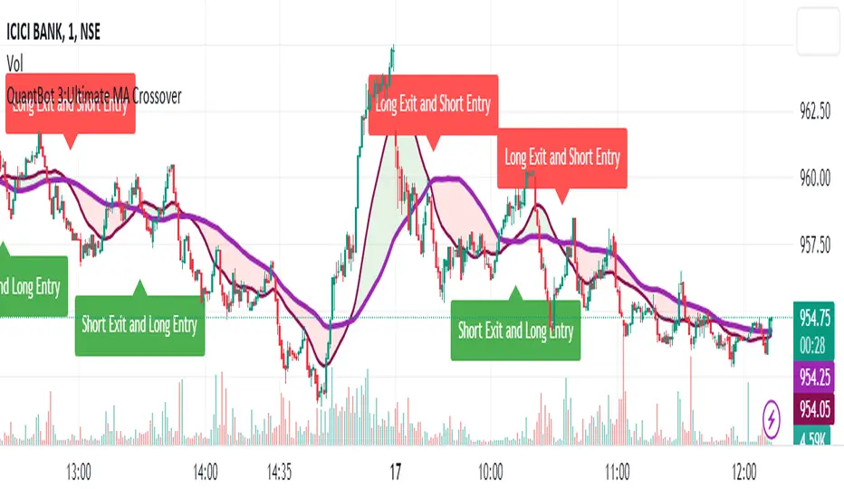
QuantBot 3:Ultimate MA CrossoverTHIS IS A SAMPLE CODE TO AUTOMATE WITH QUANTBOT
The moving average strategy is a popular and widely used technique in financial analysis and trading. It involves the calculation and analysis of moving averages, which are mathematical indicators that smooth out price data over a specified period. This strategy is primarily applied in the context of stock trading, but it can be used for other financial instruments as well.
The concept behind the moving average strategy is to identify trends and potential entry or exit points in the market. By calculating and analyzing moving averages of different timeframes, traders aim to capture the overall direction of the price movement and filter out short-term fluctuations or noise.
To implement the moving average strategy, a trader typically selects two or more moving averages with different periods. The most common combinations include the 50-day and 200-day moving averages. The shorter-term moving average is considered more reactive to price changes, while the longer-term moving average provides a smoother trend line. When the shorter-term moving average crosses above the longer-term moving average, it generates a buy signal, indicating a potential upward trend. Conversely, when the shorter-term moving average crosses below the longer-term moving average, it generates a sell signal, indicating a potential downward trend.
Traders can use various variations of the moving average strategy based on their trading objectives and risk tolerance. For instance, some traders may prefer to use exponential moving averages (EMAs) instead of simple moving averages (SMAs) to give more weight to recent price data. Others may incorporate additional indicators or filters to confirm signals or avoid false signals.
One of the strengths of the moving average strategy is its simplicity and ease of interpretation. It provides a clear visual representation of the trend direction and potential entry or exit points. However, it's important to note that the moving average strategy is a lagging indicator, meaning that it relies on past price data. Therefore, it may not always accurately predict future market movements or capture sudden reversals.
Like any trading strategy, the moving average strategy is not foolproof and carries risks. It is crucial for traders to conduct thorough analysis, consider other relevant factors, and manage their risk through proper position sizing and risk management techniques. Additionally, it's important to adapt the strategy to specific market conditions and combine it with other complementary strategies or indicators for improved decision-making.
Overall, the moving average strategy serves as a valuable tool for traders to identify and follow trends in financial markets, aiding in the analysis of price movements and potential trading opportunities.
Goertzel Cycle Composite Wave [Loxx]As the financial markets become increasingly complex and data-driven, traders and analysts must leverage powerful tools to gain insights and make informed decisions. One such tool is the Goertzel Cycle Composite Wave indicator, a sophisticated technical analysis indicator that helps identify cyclical patterns in financial data. This powerful tool is capable of detecting cyclical patterns in financial data, helping traders to make better predictions and optimize their trading strategies. With its unique combination of mathematical algorithms and advanced charting capabilities, this indicator has the potential to revolutionize the way we approach financial modeling and trading.
*** To decrease the load time of this indicator, only XX many bars back will render to the chart. You can control this value with the setting "Number of Bars to Render". This doesn't have anything to do with repainting or the indicator being endpointed***
█ Brief Overview of the Goertzel Cycle Composite Wave
The Goertzel Cycle Composite Wave is a sophisticated technical analysis tool that utilizes the Goertzel algorithm to analyze and visualize cyclical components within a financial time series. By identifying these cycles and their characteristics, the indicator aims to provide valuable insights into the market's underlying price movements, which could potentially be used for making informed trading decisions.
The Goertzel Cycle Composite Wave is considered a non-repainting and endpointed indicator. This means that once a value has been calculated for a specific bar, that value will not change in subsequent bars, and the indicator is designed to have a clear start and end point. This is an important characteristic for indicators used in technical analysis, as it allows traders to make informed decisions based on historical data without the risk of hindsight bias or future changes in the indicator's values. This means traders can use this indicator trading purposes.
The repainting version of this indicator with forecasting, cycle selection/elimination options, and data output table can be found here:
Goertzel Browser
The primary purpose of this indicator is to:
1. Detect and analyze the dominant cycles present in the price data.
2. Reconstruct and visualize the composite wave based on the detected cycles.
To achieve this, the indicator performs several tasks:
1. Detrending the price data: The indicator preprocesses the price data using various detrending techniques, such as Hodrick-Prescott filters, zero-lag moving averages, and linear regression, to remove the underlying trend and focus on the cyclical components.
2. Applying the Goertzel algorithm: The indicator applies the Goertzel algorithm to the detrended price data, identifying the dominant cycles and their characteristics, such as amplitude, phase, and cycle strength.
3. Constructing the composite wave: The indicator reconstructs the composite wave by combining the detected cycles, either by using a user-defined list of cycles or by selecting the top N cycles based on their amplitude or cycle strength.
4. Visualizing the composite wave: The indicator plots the composite wave, using solid lines for the cycles. The color of the lines indicates whether the wave is increasing or decreasing.
This indicator is a powerful tool that employs the Goertzel algorithm to analyze and visualize the cyclical components within a financial time series. By providing insights into the underlying price movements, the indicator aims to assist traders in making more informed decisions.
█ What is the Goertzel Algorithm?
The Goertzel algorithm, named after Gerald Goertzel, is a digital signal processing technique that is used to efficiently compute individual terms of the Discrete Fourier Transform (DFT). It was first introduced in 1958, and since then, it has found various applications in the fields of engineering, mathematics, and physics.
The Goertzel algorithm is primarily used to detect specific frequency components within a digital signal, making it particularly useful in applications where only a few frequency components are of interest. The algorithm is computationally efficient, as it requires fewer calculations than the Fast Fourier Transform (FFT) when detecting a small number of frequency components. This efficiency makes the Goertzel algorithm a popular choice in applications such as:
1. Telecommunications: The Goertzel algorithm is used for decoding Dual-Tone Multi-Frequency (DTMF) signals, which are the tones generated when pressing buttons on a telephone keypad. By identifying specific frequency components, the algorithm can accurately determine which button has been pressed.
2. Audio processing: The algorithm can be used to detect specific pitches or harmonics in an audio signal, making it useful in applications like pitch detection and tuning musical instruments.
3. Vibration analysis: In the field of mechanical engineering, the Goertzel algorithm can be applied to analyze vibrations in rotating machinery, helping to identify faulty components or signs of wear.
4. Power system analysis: The algorithm can be used to measure harmonic content in power systems, allowing engineers to assess power quality and detect potential issues.
The Goertzel algorithm is used in these applications because it offers several advantages over other methods, such as the FFT:
1. Computational efficiency: The Goertzel algorithm requires fewer calculations when detecting a small number of frequency components, making it more computationally efficient than the FFT in these cases.
2. Real-time analysis: The algorithm can be implemented in a streaming fashion, allowing for real-time analysis of signals, which is crucial in applications like telecommunications and audio processing.
3. Memory efficiency: The Goertzel algorithm requires less memory than the FFT, as it only computes the frequency components of interest.
4. Precision: The algorithm is less susceptible to numerical errors compared to the FFT, ensuring more accurate results in applications where precision is essential.
The Goertzel algorithm is an efficient digital signal processing technique that is primarily used to detect specific frequency components within a signal. Its computational efficiency, real-time capabilities, and precision make it an attractive choice for various applications, including telecommunications, audio processing, vibration analysis, and power system analysis. The algorithm has been widely adopted since its introduction in 1958 and continues to be an essential tool in the fields of engineering, mathematics, and physics.
█ Goertzel Algorithm in Quantitative Finance: In-Depth Analysis and Applications
The Goertzel algorithm, initially designed for signal processing in telecommunications, has gained significant traction in the financial industry due to its efficient frequency detection capabilities. In quantitative finance, the Goertzel algorithm has been utilized for uncovering hidden market cycles, developing data-driven trading strategies, and optimizing risk management. This section delves deeper into the applications of the Goertzel algorithm in finance, particularly within the context of quantitative trading and analysis.
Unveiling Hidden Market Cycles:
Market cycles are prevalent in financial markets and arise from various factors, such as economic conditions, investor psychology, and market participant behavior. The Goertzel algorithm's ability to detect and isolate specific frequencies in price data helps trader analysts identify hidden market cycles that may otherwise go unnoticed. By examining the amplitude, phase, and periodicity of each cycle, traders can better understand the underlying market structure and dynamics, enabling them to develop more informed and effective trading strategies.
Developing Quantitative Trading Strategies:
The Goertzel algorithm's versatility allows traders to incorporate its insights into a wide range of trading strategies. By identifying the dominant market cycles in a financial instrument's price data, traders can create data-driven strategies that capitalize on the cyclical nature of markets.
For instance, a trader may develop a mean-reversion strategy that takes advantage of the identified cycles. By establishing positions when the price deviates from the predicted cycle, the trader can profit from the subsequent reversion to the cycle's mean. Similarly, a momentum-based strategy could be designed to exploit the persistence of a dominant cycle by entering positions that align with the cycle's direction.
Enhancing Risk Management:
The Goertzel algorithm plays a vital role in risk management for quantitative strategies. By analyzing the cyclical components of a financial instrument's price data, traders can gain insights into the potential risks associated with their trading strategies.
By monitoring the amplitude and phase of dominant cycles, a trader can detect changes in market dynamics that may pose risks to their positions. For example, a sudden increase in amplitude may indicate heightened volatility, prompting the trader to adjust position sizing or employ hedging techniques to protect their portfolio. Additionally, changes in phase alignment could signal a potential shift in market sentiment, necessitating adjustments to the trading strategy.
Expanding Quantitative Toolkits:
Traders can augment the Goertzel algorithm's insights by combining it with other quantitative techniques, creating a more comprehensive and sophisticated analysis framework. For example, machine learning algorithms, such as neural networks or support vector machines, could be trained on features extracted from the Goertzel algorithm to predict future price movements more accurately.
Furthermore, the Goertzel algorithm can be integrated with other technical analysis tools, such as moving averages or oscillators, to enhance their effectiveness. By applying these tools to the identified cycles, traders can generate more robust and reliable trading signals.
The Goertzel algorithm offers invaluable benefits to quantitative finance practitioners by uncovering hidden market cycles, aiding in the development of data-driven trading strategies, and improving risk management. By leveraging the insights provided by the Goertzel algorithm and integrating it with other quantitative techniques, traders can gain a deeper understanding of market dynamics and devise more effective trading strategies.
█ Indicator Inputs
src: This is the source data for the analysis, typically the closing price of the financial instrument.
detrendornot: This input determines the method used for detrending the source data. Detrending is the process of removing the underlying trend from the data to focus on the cyclical components.
The available options are:
hpsmthdt: Detrend using Hodrick-Prescott filter centered moving average.
zlagsmthdt: Detrend using zero-lag moving average centered moving average.
logZlagRegression: Detrend using logarithmic zero-lag linear regression.
hpsmth: Detrend using Hodrick-Prescott filter.
zlagsmth: Detrend using zero-lag moving average.
DT_HPper1 and DT_HPper2: These inputs define the period range for the Hodrick-Prescott filter centered moving average when detrendornot is set to hpsmthdt.
DT_ZLper1 and DT_ZLper2: These inputs define the period range for the zero-lag moving average centered moving average when detrendornot is set to zlagsmthdt.
DT_RegZLsmoothPer: This input defines the period for the zero-lag moving average used in logarithmic zero-lag linear regression when detrendornot is set to logZlagRegression.
HPsmoothPer: This input defines the period for the Hodrick-Prescott filter when detrendornot is set to hpsmth.
ZLMAsmoothPer: This input defines the period for the zero-lag moving average when detrendornot is set to zlagsmth.
MaxPer: This input sets the maximum period for the Goertzel algorithm to search for cycles.
squaredAmp: This boolean input determines whether the amplitude should be squared in the Goertzel algorithm.
useAddition: This boolean input determines whether the Goertzel algorithm should use addition for combining the cycles.
useCosine: This boolean input determines whether the Goertzel algorithm should use cosine waves instead of sine waves.
UseCycleStrength: This boolean input determines whether the Goertzel algorithm should compute the cycle strength, which is a normalized measure of the cycle's amplitude.
WindowSizePast: These inputs define the window size for the composite wave.
FilterBartels: This boolean input determines whether Bartel's test should be applied to filter out non-significant cycles.
BartNoCycles: This input sets the number of cycles to be used in Bartel's test.
BartSmoothPer: This input sets the period for the moving average used in Bartel's test.
BartSigLimit: This input sets the significance limit for Bartel's test, below which cycles are considered insignificant.
SortBartels: This boolean input determines whether the cycles should be sorted by their Bartel's test results.
StartAtCycle: This input determines the starting index for selecting the top N cycles when UseCycleList is set to false. This allows you to skip a certain number of cycles from the top before selecting the desired number of cycles.
UseTopCycles: This input sets the number of top cycles to use for constructing the composite wave when UseCycleList is set to false. The cycles are ranked based on their amplitudes or cycle strengths, depending on the UseCycleStrength input.
SubtractNoise: This boolean input determines whether to subtract the noise (remaining cycles) from the composite wave. If set to true, the composite wave will only include the top N cycles specified by UseTopCycles.
█ Exploring Auxiliary Functions
The following functions demonstrate advanced techniques for analyzing financial markets, including zero-lag moving averages, Bartels probability, detrending, and Hodrick-Prescott filtering. This section examines each function in detail, explaining their purpose, methodology, and applications in finance. We will examine how each function contributes to the overall performance and effectiveness of the indicator and how they work together to create a powerful analytical tool.
Zero-Lag Moving Average:
The zero-lag moving average function is designed to minimize the lag typically associated with moving averages. This is achieved through a two-step weighted linear regression process that emphasizes more recent data points. The function calculates a linearly weighted moving average (LWMA) on the input data and then applies another LWMA on the result. By doing this, the function creates a moving average that closely follows the price action, reducing the lag and improving the responsiveness of the indicator.
The zero-lag moving average function is used in the indicator to provide a responsive, low-lag smoothing of the input data. This function helps reduce the noise and fluctuations in the data, making it easier to identify and analyze underlying trends and patterns. By minimizing the lag associated with traditional moving averages, this function allows the indicator to react more quickly to changes in market conditions, providing timely signals and improving the overall effectiveness of the indicator.
Bartels Probability:
The Bartels probability function calculates the probability of a given cycle being significant in a time series. It uses a mathematical test called the Bartels test to assess the significance of cycles detected in the data. The function calculates coefficients for each detected cycle and computes an average amplitude and an expected amplitude. By comparing these values, the Bartels probability is derived, indicating the likelihood of a cycle's significance. This information can help in identifying and analyzing dominant cycles in financial markets.
The Bartels probability function is incorporated into the indicator to assess the significance of detected cycles in the input data. By calculating the Bartels probability for each cycle, the indicator can prioritize the most significant cycles and focus on the market dynamics that are most relevant to the current trading environment. This function enhances the indicator's ability to identify dominant market cycles, improving its predictive power and aiding in the development of effective trading strategies.
Detrend Logarithmic Zero-Lag Regression:
The detrend logarithmic zero-lag regression function is used for detrending data while minimizing lag. It combines a zero-lag moving average with a linear regression detrending method. The function first calculates the zero-lag moving average of the logarithm of input data and then applies a linear regression to remove the trend. By detrending the data, the function isolates the cyclical components, making it easier to analyze and interpret the underlying market dynamics.
The detrend logarithmic zero-lag regression function is used in the indicator to isolate the cyclical components of the input data. By detrending the data, the function enables the indicator to focus on the cyclical movements in the market, making it easier to analyze and interpret market dynamics. This function is essential for identifying cyclical patterns and understanding the interactions between different market cycles, which can inform trading decisions and enhance overall market understanding.
Bartels Cycle Significance Test:
The Bartels cycle significance test is a function that combines the Bartels probability function and the detrend logarithmic zero-lag regression function to assess the significance of detected cycles. The function calculates the Bartels probability for each cycle and stores the results in an array. By analyzing the probability values, traders and analysts can identify the most significant cycles in the data, which can be used to develop trading strategies and improve market understanding.
The Bartels cycle significance test function is integrated into the indicator to provide a comprehensive analysis of the significance of detected cycles. By combining the Bartels probability function and the detrend logarithmic zero-lag regression function, this test evaluates the significance of each cycle and stores the results in an array. The indicator can then use this information to prioritize the most significant cycles and focus on the most relevant market dynamics. This function enhances the indicator's ability to identify and analyze dominant market cycles, providing valuable insights for trading and market analysis.
Hodrick-Prescott Filter:
The Hodrick-Prescott filter is a popular technique used to separate the trend and cyclical components of a time series. The function applies a smoothing parameter to the input data and calculates a smoothed series using a two-sided filter. This smoothed series represents the trend component, which can be subtracted from the original data to obtain the cyclical component. The Hodrick-Prescott filter is commonly used in economics and finance to analyze economic data and financial market trends.
The Hodrick-Prescott filter is incorporated into the indicator to separate the trend and cyclical components of the input data. By applying the filter to the data, the indicator can isolate the trend component, which can be used to analyze long-term market trends and inform trading decisions. Additionally, the cyclical component can be used to identify shorter-term market dynamics and provide insights into potential trading opportunities. The inclusion of the Hodrick-Prescott filter adds another layer of analysis to the indicator, making it more versatile and comprehensive.
Detrending Options: Detrend Centered Moving Average:
The detrend centered moving average function provides different detrending methods, including the Hodrick-Prescott filter and the zero-lag moving average, based on the selected detrending method. The function calculates two sets of smoothed values using the chosen method and subtracts one set from the other to obtain a detrended series. By offering multiple detrending options, this function allows traders and analysts to select the most appropriate method for their specific needs and preferences.
The detrend centered moving average function is integrated into the indicator to provide users with multiple detrending options, including the Hodrick-Prescott filter and the zero-lag moving average. By offering multiple detrending methods, the indicator allows users to customize the analysis to their specific needs and preferences, enhancing the indicator's overall utility and adaptability. This function ensures that the indicator can cater to a wide range of trading styles and objectives, making it a valuable tool for a diverse group of market participants.
The auxiliary functions functions discussed in this section demonstrate the power and versatility of mathematical techniques in analyzing financial markets. By understanding and implementing these functions, traders and analysts can gain valuable insights into market dynamics, improve their trading strategies, and make more informed decisions. The combination of zero-lag moving averages, Bartels probability, detrending methods, and the Hodrick-Prescott filter provides a comprehensive toolkit for analyzing and interpreting financial data. The integration of advanced functions in a financial indicator creates a powerful and versatile analytical tool that can provide valuable insights into financial markets. By combining the zero-lag moving average,
█ In-Depth Analysis of the Goertzel Cycle Composite Wave Code
The Goertzel Cycle Composite Wave code is an implementation of the Goertzel Algorithm, an efficient technique to perform spectral analysis on a signal. The code is designed to detect and analyze dominant cycles within a given financial market data set. This section will provide an extremely detailed explanation of the code, its structure, functions, and intended purpose.
Function signature and input parameters:
The Goertzel Cycle Composite Wave function accepts numerous input parameters for customization, including source data (src), the current bar (forBar), sample size (samplesize), period (per), squared amplitude flag (squaredAmp), addition flag (useAddition), cosine flag (useCosine), cycle strength flag (UseCycleStrength), past sizes (WindowSizePast), Bartels filter flag (FilterBartels), Bartels-related parameters (BartNoCycles, BartSmoothPer, BartSigLimit), sorting flag (SortBartels), and output buffers (goeWorkPast, cyclebuffer, amplitudebuffer, phasebuffer, cycleBartelsBuffer).
Initializing variables and arrays:
The code initializes several float arrays (goeWork1, goeWork2, goeWork3, goeWork4) with the same length as twice the period (2 * per). These arrays store intermediate results during the execution of the algorithm.
Preprocessing input data:
The input data (src) undergoes preprocessing to remove linear trends. This step enhances the algorithm's ability to focus on cyclical components in the data. The linear trend is calculated by finding the slope between the first and last values of the input data within the sample.
Iterative calculation of Goertzel coefficients:
The core of the Goertzel Cycle Composite Wave algorithm lies in the iterative calculation of Goertzel coefficients for each frequency bin. These coefficients represent the spectral content of the input data at different frequencies. The code iterates through the range of frequencies, calculating the Goertzel coefficients using a nested loop structure.
Cycle strength computation:
The code calculates the cycle strength based on the Goertzel coefficients. This is an optional step, controlled by the UseCycleStrength flag. The cycle strength provides information on the relative influence of each cycle on the data per bar, considering both amplitude and cycle length. The algorithm computes the cycle strength either by squaring the amplitude (controlled by squaredAmp flag) or using the actual amplitude values.
Phase calculation:
The Goertzel Cycle Composite Wave code computes the phase of each cycle, which represents the position of the cycle within the input data. The phase is calculated using the arctangent function (math.atan) based on the ratio of the imaginary and real components of the Goertzel coefficients.
Peak detection and cycle extraction:
The algorithm performs peak detection on the computed amplitudes or cycle strengths to identify dominant cycles. It stores the detected cycles in the cyclebuffer array, along with their corresponding amplitudes and phases in the amplitudebuffer and phasebuffer arrays, respectively.
Sorting cycles by amplitude or cycle strength:
The code sorts the detected cycles based on their amplitude or cycle strength in descending order. This allows the algorithm to prioritize cycles with the most significant impact on the input data.
Bartels cycle significance test:
If the FilterBartels flag is set, the code performs a Bartels cycle significance test on the detected cycles. This test determines the statistical significance of each cycle and filters out the insignificant cycles. The significant cycles are stored in the cycleBartelsBuffer array. If the SortBartels flag is set, the code sorts the significant cycles based on their Bartels significance values.
Waveform calculation:
The Goertzel Cycle Composite Wave code calculates the waveform of the significant cycles for specified time windows. The windows are defined by the WindowSizePast parameters, respectively. The algorithm uses either cosine or sine functions (controlled by the useCosine flag) to calculate the waveforms for each cycle. The useAddition flag determines whether the waveforms should be added or subtracted.
Storing waveforms in a matrix:
The calculated waveforms for the cycle is stored in the matrix - goeWorkPast. This matrix holds the waveforms for the specified time windows. Each row in the matrix represents a time window position, and each column corresponds to a cycle.
Returning the number of cycles:
The Goertzel Cycle Composite Wave function returns the total number of detected cycles (number_of_cycles) after processing the input data. This information can be used to further analyze the results or to visualize the detected cycles.
The Goertzel Cycle Composite Wave code is a comprehensive implementation of the Goertzel Algorithm, specifically designed for detecting and analyzing dominant cycles within financial market data. The code offers a high level of customization, allowing users to fine-tune the algorithm based on their specific needs. The Goertzel Cycle Composite Wave's combination of preprocessing, iterative calculations, cycle extraction, sorting, significance testing, and waveform calculation makes it a powerful tool for understanding cyclical components in financial data.
█ Generating and Visualizing Composite Waveform
The indicator calculates and visualizes the composite waveform for specified time windows based on the detected cycles. Here's a detailed explanation of this process:
Updating WindowSizePast:
The WindowSizePast is updated to ensure they are at least twice the MaxPer (maximum period).
Initializing matrices and arrays:
The matrix goeWorkPast is initialized to store the Goertzel results for specified time windows. Multiple arrays are also initialized to store cycle, amplitude, phase, and Bartels information.
Preparing the source data (srcVal) array:
The source data is copied into an array, srcVal, and detrended using one of the selected methods (hpsmthdt, zlagsmthdt, logZlagRegression, hpsmth, or zlagsmth).
Goertzel function call:
The Goertzel function is called to analyze the detrended source data and extract cycle information. The output, number_of_cycles, contains the number of detected cycles.
Initializing arrays for waveforms:
The goertzel array is initialized to store the endpoint Goertzel.
Calculating composite waveform (goertzel array):
The composite waveform is calculated by summing the selected cycles (either from the user-defined cycle list or the top cycles) and optionally subtracting the noise component.
Drawing composite waveform (pvlines):
The composite waveform is drawn on the chart using solid lines. The color of the lines is determined by the direction of the waveform (green for upward, red for downward).
To summarize, this indicator generates a composite waveform based on the detected cycles in the financial data. It calculates the composite waveforms and visualizes them on the chart using colored lines.
█ Enhancing the Goertzel Algorithm-Based Script for Financial Modeling and Trading
The Goertzel algorithm-based script for detecting dominant cycles in financial data is a powerful tool for financial modeling and trading. It provides valuable insights into the past behavior of these cycles. However, as with any algorithm, there is always room for improvement. This section discusses potential enhancements to the existing script to make it even more robust and versatile for financial modeling, general trading, advanced trading, and high-frequency finance trading.
Enhancements for Financial Modeling
Data preprocessing: One way to improve the script's performance for financial modeling is to introduce more advanced data preprocessing techniques. This could include removing outliers, handling missing data, and normalizing the data to ensure consistent and accurate results.
Additional detrending and smoothing methods: Incorporating more sophisticated detrending and smoothing techniques, such as wavelet transform or empirical mode decomposition, can help improve the script's ability to accurately identify cycles and trends in the data.
Machine learning integration: Integrating machine learning techniques, such as artificial neural networks or support vector machines, can help enhance the script's predictive capabilities, leading to more accurate financial models.
Enhancements for General and Advanced Trading
Customizable indicator integration: Allowing users to integrate their own technical indicators can help improve the script's effectiveness for both general and advanced trading. By enabling the combination of the dominant cycle information with other technical analysis tools, traders can develop more comprehensive trading strategies.
Risk management and position sizing: Incorporating risk management and position sizing functionality into the script can help traders better manage their trades and control potential losses. This can be achieved by calculating the optimal position size based on the user's risk tolerance and account size.
Multi-timeframe analysis: Enhancing the script to perform multi-timeframe analysis can provide traders with a more holistic view of market trends and cycles. By identifying dominant cycles on different timeframes, traders can gain insights into the potential confluence of cycles and make better-informed trading decisions.
Enhancements for High-Frequency Finance Trading
Algorithm optimization: To ensure the script's suitability for high-frequency finance trading, optimizing the algorithm for faster execution is crucial. This can be achieved by employing efficient data structures and refining the calculation methods to minimize computational complexity.
Real-time data streaming: Integrating real-time data streaming capabilities into the script can help high-frequency traders react to market changes more quickly. By continuously updating the cycle information based on real-time market data, traders can adapt their strategies accordingly and capitalize on short-term market fluctuations.
Order execution and trade management: To fully leverage the script's capabilities for high-frequency trading, implementing functionality for automated order execution and trade management is essential. This can include features such as stop-loss and take-profit orders, trailing stops, and automated trade exit strategies.
While the existing Goertzel algorithm-based script is a valuable tool for detecting dominant cycles in financial data, there are several potential enhancements that can make it even more powerful for financial modeling, general trading, advanced trading, and high-frequency finance trading. By incorporating these improvements, the script can become a more versatile and effective tool for traders and financial analysts alike.
█ Understanding the Limitations of the Goertzel Algorithm
While the Goertzel algorithm-based script for detecting dominant cycles in financial data provides valuable insights, it is important to be aware of its limitations and drawbacks. Some of the key drawbacks of this indicator are:
Lagging nature:
As with many other technical indicators, the Goertzel algorithm-based script can suffer from lagging effects, meaning that it may not immediately react to real-time market changes. This lag can lead to late entries and exits, potentially resulting in reduced profitability or increased losses.
Parameter sensitivity:
The performance of the script can be sensitive to the chosen parameters, such as the detrending methods, smoothing techniques, and cycle detection settings. Improper parameter selection may lead to inaccurate cycle detection or increased false signals, which can negatively impact trading performance.
Complexity:
The Goertzel algorithm itself is relatively complex, making it difficult for novice traders or those unfamiliar with the concept of cycle analysis to fully understand and effectively utilize the script. This complexity can also make it challenging to optimize the script for specific trading styles or market conditions.
Overfitting risk:
As with any data-driven approach, there is a risk of overfitting when using the Goertzel algorithm-based script. Overfitting occurs when a model becomes too specific to the historical data it was trained on, leading to poor performance on new, unseen data. This can result in misleading signals and reduced trading performance.
Limited applicability:
The Goertzel algorithm-based script may not be suitable for all markets, trading styles, or timeframes. Its effectiveness in detecting cycles may be limited in certain market conditions, such as during periods of extreme volatility or low liquidity.
While the Goertzel algorithm-based script offers valuable insights into dominant cycles in financial data, it is essential to consider its drawbacks and limitations when incorporating it into a trading strategy. Traders should always use the script in conjunction with other technical and fundamental analysis tools, as well as proper risk management, to make well-informed trading decisions.
█ Interpreting Results
The Goertzel Cycle Composite Wave indicator can be interpreted by analyzing the plotted lines. The indicator plots two lines: composite waves. The composite wave represents the composite wave of the price data.
The composite wave line displays a solid line, with green indicating a bullish trend and red indicating a bearish trend.
Interpreting the Goertzel Cycle Composite Wave indicator involves identifying the trend of the composite wave lines and matching them with the corresponding bullish or bearish color.
█ Conclusion
The Goertzel Cycle Composite Wave indicator is a powerful tool for identifying and analyzing cyclical patterns in financial markets. Its ability to detect multiple cycles of varying frequencies and strengths make it a valuable addition to any trader's technical analysis toolkit. However, it is important to keep in mind that the Goertzel Cycle Composite Wave indicator should be used in conjunction with other technical analysis tools and fundamental analysis to achieve the best results. With continued refinement and development, the Goertzel Cycle Composite Wave indicator has the potential to become a highly effective tool for financial modeling, general trading, advanced trading, and high-frequency finance trading. Its accuracy and versatility make it a promising candidate for further research and development.
█ Footnotes
What is the Bartels Test for Cycle Significance?
The Bartels Cycle Significance Test is a statistical method that determines whether the peaks and troughs of a time series are statistically significant. The test is named after its inventor, George Bartels, who developed it in the mid-20th century.
The Bartels test is designed to analyze the cyclical components of a time series, which can help traders and analysts identify trends and cycles in financial markets. The test calculates a Bartels statistic, which measures the degree of non-randomness or autocorrelation in the time series.
The Bartels statistic is calculated by first splitting the time series into two halves and calculating the range of the peaks and troughs in each half. The test then compares these ranges using a t-test, which measures the significance of the difference between the two ranges.
If the Bartels statistic is greater than a critical value, it indicates that the peaks and troughs in the time series are non-random and that there is a significant cyclical component to the data. Conversely, if the Bartels statistic is less than the critical value, it suggests that the peaks and troughs are random and that there is no significant cyclical component.
The Bartels Cycle Significance Test is particularly useful in financial analysis because it can help traders and analysts identify significant cycles in asset prices, which can in turn inform investment decisions. However, it is important to note that the test is not perfect and can produce false signals in certain situations, particularly in noisy or volatile markets. Therefore, it is always recommended to use the test in conjunction with other technical and fundamental indicators to confirm trends and cycles.
Deep-dive into the Hodrick-Prescott Fitler
The Hodrick-Prescott (HP) filter is a statistical tool used in economics and finance to separate a time series into two components: a trend component and a cyclical component. It is a powerful tool for identifying long-term trends in economic and financial data and is widely used by economists, central banks, and financial institutions around the world.
The HP filter was first introduced in the 1990s by economists Robert Hodrick and Edward Prescott. It is a simple, two-parameter filter that separates a time series into a trend component and a cyclical component. The trend component represents the long-term behavior of the data, while the cyclical component captures the shorter-term fluctuations around the trend.
The HP filter works by minimizing the following objective function:
Minimize: (Sum of Squared Deviations) + λ (Sum of Squared Second Differences)
Where:
1. The first term represents the deviation of the data from the trend.
2. The second term represents the smoothness of the trend.
3. λ is a smoothing parameter that determines the degree of smoothness of the trend.
The smoothing parameter λ is typically set to a value between 100 and 1600, depending on the frequency of the data. Higher values of λ lead to a smoother trend, while lower values lead to a more volatile trend.
The HP filter has several advantages over other smoothing techniques. It is a non-parametric method, meaning that it does not make any assumptions about the underlying distribution of the data. It also allows for easy comparison of trends across different time series and can be used with data of any frequency.
However, the HP filter also has some limitations. It assumes that the trend is a smooth function, which may not be the case in some situations. It can also be sensitive to changes in the smoothing parameter λ, which may result in different trends for the same data. Additionally, the filter may produce unrealistic trends for very short time series.
Despite these limitations, the HP filter remains a valuable tool for analyzing economic and financial data. It is widely used by central banks and financial institutions to monitor long-term trends in the economy, and it can be used to identify turning points in the business cycle. The filter can also be used to analyze asset prices, exchange rates, and other financial variables.
The Hodrick-Prescott filter is a powerful tool for analyzing economic and financial data. It separates a time series into a trend component and a cyclical component, allowing for easy identification of long-term trends and turning points in the business cycle. While it has some limitations, it remains a valuable tool for economists, central banks, and financial institutions around the world.

Goertzel Browser [Loxx]As the financial markets become increasingly complex and data-driven, traders and analysts must leverage powerful tools to gain insights and make informed decisions. One such tool is the Goertzel Browser indicator, a sophisticated technical analysis indicator that helps identify cyclical patterns in financial data. This powerful tool is capable of detecting cyclical patterns in financial data, helping traders to make better predictions and optimize their trading strategies. With its unique combination of mathematical algorithms and advanced charting capabilities, this indicator has the potential to revolutionize the way we approach financial modeling and trading.
█ Brief Overview of the Goertzel Browser
The Goertzel Browser is a sophisticated technical analysis tool that utilizes the Goertzel algorithm to analyze and visualize cyclical components within a financial time series. By identifying these cycles and their characteristics, the indicator aims to provide valuable insights into the market's underlying price movements, which could potentially be used for making informed trading decisions.
The primary purpose of this indicator is to:
1. Detect and analyze the dominant cycles present in the price data.
2. Reconstruct and visualize the composite wave based on the detected cycles.
3. Project the composite wave into the future, providing a potential roadmap for upcoming price movements.
To achieve this, the indicator performs several tasks:
1. Detrending the price data: The indicator preprocesses the price data using various detrending techniques, such as Hodrick-Prescott filters, zero-lag moving averages, and linear regression, to remove the underlying trend and focus on the cyclical components.
2. Applying the Goertzel algorithm: The indicator applies the Goertzel algorithm to the detrended price data, identifying the dominant cycles and their characteristics, such as amplitude, phase, and cycle strength.
3. Constructing the composite wave: The indicator reconstructs the composite wave by combining the detected cycles, either by using a user-defined list of cycles or by selecting the top N cycles based on their amplitude or cycle strength.
4. Visualizing the composite wave: The indicator plots the composite wave, using solid lines for the past and dotted lines for the future projections. The color of the lines indicates whether the wave is increasing or decreasing.
5. Displaying cycle information: The indicator provides a table that displays detailed information about the detected cycles, including their rank, period, Bartel's test results, amplitude, and phase.
This indicator is a powerful tool that employs the Goertzel algorithm to analyze and visualize the cyclical components within a financial time series. By providing insights into the underlying price movements and their potential future trajectory, the indicator aims to assist traders in making more informed decisions.
█ What is the Goertzel Algorithm?
The Goertzel algorithm, named after Gerald Goertzel, is a digital signal processing technique that is used to efficiently compute individual terms of the Discrete Fourier Transform (DFT). It was first introduced in 1958, and since then, it has found various applications in the fields of engineering, mathematics, and physics.
The Goertzel algorithm is primarily used to detect specific frequency components within a digital signal, making it particularly useful in applications where only a few frequency components are of interest. The algorithm is computationally efficient, as it requires fewer calculations than the Fast Fourier Transform (FFT) when detecting a small number of frequency components. This efficiency makes the Goertzel algorithm a popular choice in applications such as:
1. Telecommunications: The Goertzel algorithm is used for decoding Dual-Tone Multi-Frequency (DTMF) signals, which are the tones generated when pressing buttons on a telephone keypad. By identifying specific frequency components, the algorithm can accurately determine which button has been pressed.
2. Audio processing: The algorithm can be used to detect specific pitches or harmonics in an audio signal, making it useful in applications like pitch detection and tuning musical instruments.
3. Vibration analysis: In the field of mechanical engineering, the Goertzel algorithm can be applied to analyze vibrations in rotating machinery, helping to identify faulty components or signs of wear.
4. Power system analysis: The algorithm can be used to measure harmonic content in power systems, allowing engineers to assess power quality and detect potential issues.
The Goertzel algorithm is used in these applications because it offers several advantages over other methods, such as the FFT:
1. Computational efficiency: The Goertzel algorithm requires fewer calculations when detecting a small number of frequency components, making it more computationally efficient than the FFT in these cases.
2. Real-time analysis: The algorithm can be implemented in a streaming fashion, allowing for real-time analysis of signals, which is crucial in applications like telecommunications and audio processing.
3. Memory efficiency: The Goertzel algorithm requires less memory than the FFT, as it only computes the frequency components of interest.
4. Precision: The algorithm is less susceptible to numerical errors compared to the FFT, ensuring more accurate results in applications where precision is essential.
The Goertzel algorithm is an efficient digital signal processing technique that is primarily used to detect specific frequency components within a signal. Its computational efficiency, real-time capabilities, and precision make it an attractive choice for various applications, including telecommunications, audio processing, vibration analysis, and power system analysis. The algorithm has been widely adopted since its introduction in 1958 and continues to be an essential tool in the fields of engineering, mathematics, and physics.
█ Goertzel Algorithm in Quantitative Finance: In-Depth Analysis and Applications
The Goertzel algorithm, initially designed for signal processing in telecommunications, has gained significant traction in the financial industry due to its efficient frequency detection capabilities. In quantitative finance, the Goertzel algorithm has been utilized for uncovering hidden market cycles, developing data-driven trading strategies, and optimizing risk management. This section delves deeper into the applications of the Goertzel algorithm in finance, particularly within the context of quantitative trading and analysis.
Unveiling Hidden Market Cycles:
Market cycles are prevalent in financial markets and arise from various factors, such as economic conditions, investor psychology, and market participant behavior. The Goertzel algorithm's ability to detect and isolate specific frequencies in price data helps trader analysts identify hidden market cycles that may otherwise go unnoticed. By examining the amplitude, phase, and periodicity of each cycle, traders can better understand the underlying market structure and dynamics, enabling them to develop more informed and effective trading strategies.
Developing Quantitative Trading Strategies:
The Goertzel algorithm's versatility allows traders to incorporate its insights into a wide range of trading strategies. By identifying the dominant market cycles in a financial instrument's price data, traders can create data-driven strategies that capitalize on the cyclical nature of markets.
For instance, a trader may develop a mean-reversion strategy that takes advantage of the identified cycles. By establishing positions when the price deviates from the predicted cycle, the trader can profit from the subsequent reversion to the cycle's mean. Similarly, a momentum-based strategy could be designed to exploit the persistence of a dominant cycle by entering positions that align with the cycle's direction.
Enhancing Risk Management:
The Goertzel algorithm plays a vital role in risk management for quantitative strategies. By analyzing the cyclical components of a financial instrument's price data, traders can gain insights into the potential risks associated with their trading strategies.
By monitoring the amplitude and phase of dominant cycles, a trader can detect changes in market dynamics that may pose risks to their positions. For example, a sudden increase in amplitude may indicate heightened volatility, prompting the trader to adjust position sizing or employ hedging techniques to protect their portfolio. Additionally, changes in phase alignment could signal a potential shift in market sentiment, necessitating adjustments to the trading strategy.
Expanding Quantitative Toolkits:
Traders can augment the Goertzel algorithm's insights by combining it with other quantitative techniques, creating a more comprehensive and sophisticated analysis framework. For example, machine learning algorithms, such as neural networks or support vector machines, could be trained on features extracted from the Goertzel algorithm to predict future price movements more accurately.
Furthermore, the Goertzel algorithm can be integrated with other technical analysis tools, such as moving averages or oscillators, to enhance their effectiveness. By applying these tools to the identified cycles, traders can generate more robust and reliable trading signals.
The Goertzel algorithm offers invaluable benefits to quantitative finance practitioners by uncovering hidden market cycles, aiding in the development of data-driven trading strategies, and improving risk management. By leveraging the insights provided by the Goertzel algorithm and integrating it with other quantitative techniques, traders can gain a deeper understanding of market dynamics and devise more effective trading strategies.
█ Indicator Inputs
src: This is the source data for the analysis, typically the closing price of the financial instrument.
detrendornot: This input determines the method used for detrending the source data. Detrending is the process of removing the underlying trend from the data to focus on the cyclical components.
The available options are:
hpsmthdt: Detrend using Hodrick-Prescott filter centered moving average.
zlagsmthdt: Detrend using zero-lag moving average centered moving average.
logZlagRegression: Detrend using logarithmic zero-lag linear regression.
hpsmth: Detrend using Hodrick-Prescott filter.
zlagsmth: Detrend using zero-lag moving average.
DT_HPper1 and DT_HPper2: These inputs define the period range for the Hodrick-Prescott filter centered moving average when detrendornot is set to hpsmthdt.
DT_ZLper1 and DT_ZLper2: These inputs define the period range for the zero-lag moving average centered moving average when detrendornot is set to zlagsmthdt.
DT_RegZLsmoothPer: This input defines the period for the zero-lag moving average used in logarithmic zero-lag linear regression when detrendornot is set to logZlagRegression.
HPsmoothPer: This input defines the period for the Hodrick-Prescott filter when detrendornot is set to hpsmth.
ZLMAsmoothPer: This input defines the period for the zero-lag moving average when detrendornot is set to zlagsmth.
MaxPer: This input sets the maximum period for the Goertzel algorithm to search for cycles.
squaredAmp: This boolean input determines whether the amplitude should be squared in the Goertzel algorithm.
useAddition: This boolean input determines whether the Goertzel algorithm should use addition for combining the cycles.
useCosine: This boolean input determines whether the Goertzel algorithm should use cosine waves instead of sine waves.
UseCycleStrength: This boolean input determines whether the Goertzel algorithm should compute the cycle strength, which is a normalized measure of the cycle's amplitude.
WindowSizePast and WindowSizeFuture: These inputs define the window size for past and future projections of the composite wave.
FilterBartels: This boolean input determines whether Bartel's test should be applied to filter out non-significant cycles.
BartNoCycles: This input sets the number of cycles to be used in Bartel's test.
BartSmoothPer: This input sets the period for the moving average used in Bartel's test.
BartSigLimit: This input sets the significance limit for Bartel's test, below which cycles are considered insignificant.
SortBartels: This boolean input determines whether the cycles should be sorted by their Bartel's test results.
UseCycleList: This boolean input determines whether a user-defined list of cycles should be used for constructing the composite wave. If set to false, the top N cycles will be used.
Cycle1, Cycle2, Cycle3, Cycle4, and Cycle5: These inputs define the user-defined list of cycles when 'UseCycleList' is set to true. If using a user-defined list, each of these inputs represents the period of a specific cycle to include in the composite wave.
StartAtCycle: This input determines the starting index for selecting the top N cycles when UseCycleList is set to false. This allows you to skip a certain number of cycles from the top before selecting the desired number of cycles.
UseTopCycles: This input sets the number of top cycles to use for constructing the composite wave when UseCycleList is set to false. The cycles are ranked based on their amplitudes or cycle strengths, depending on the UseCycleStrength input.
SubtractNoise: This boolean input determines whether to subtract the noise (remaining cycles) from the composite wave. If set to true, the composite wave will only include the top N cycles specified by UseTopCycles.
█ Exploring Auxiliary Functions
The following functions demonstrate advanced techniques for analyzing financial markets, including zero-lag moving averages, Bartels probability, detrending, and Hodrick-Prescott filtering. This section examines each function in detail, explaining their purpose, methodology, and applications in finance. We will examine how each function contributes to the overall performance and effectiveness of the indicator and how they work together to create a powerful analytical tool.
Zero-Lag Moving Average:
The zero-lag moving average function is designed to minimize the lag typically associated with moving averages. This is achieved through a two-step weighted linear regression process that emphasizes more recent data points. The function calculates a linearly weighted moving average (LWMA) on the input data and then applies another LWMA on the result. By doing this, the function creates a moving average that closely follows the price action, reducing the lag and improving the responsiveness of the indicator.
The zero-lag moving average function is used in the indicator to provide a responsive, low-lag smoothing of the input data. This function helps reduce the noise and fluctuations in the data, making it easier to identify and analyze underlying trends and patterns. By minimizing the lag associated with traditional moving averages, this function allows the indicator to react more quickly to changes in market conditions, providing timely signals and improving the overall effectiveness of the indicator.
Bartels Probability:
The Bartels probability function calculates the probability of a given cycle being significant in a time series. It uses a mathematical test called the Bartels test to assess the significance of cycles detected in the data. The function calculates coefficients for each detected cycle and computes an average amplitude and an expected amplitude. By comparing these values, the Bartels probability is derived, indicating the likelihood of a cycle's significance. This information can help in identifying and analyzing dominant cycles in financial markets.
The Bartels probability function is incorporated into the indicator to assess the significance of detected cycles in the input data. By calculating the Bartels probability for each cycle, the indicator can prioritize the most significant cycles and focus on the market dynamics that are most relevant to the current trading environment. This function enhances the indicator's ability to identify dominant market cycles, improving its predictive power and aiding in the development of effective trading strategies.
Detrend Logarithmic Zero-Lag Regression:
The detrend logarithmic zero-lag regression function is used for detrending data while minimizing lag. It combines a zero-lag moving average with a linear regression detrending method. The function first calculates the zero-lag moving average of the logarithm of input data and then applies a linear regression to remove the trend. By detrending the data, the function isolates the cyclical components, making it easier to analyze and interpret the underlying market dynamics.
The detrend logarithmic zero-lag regression function is used in the indicator to isolate the cyclical components of the input data. By detrending the data, the function enables the indicator to focus on the cyclical movements in the market, making it easier to analyze and interpret market dynamics. This function is essential for identifying cyclical patterns and understanding the interactions between different market cycles, which can inform trading decisions and enhance overall market understanding.
Bartels Cycle Significance Test:
The Bartels cycle significance test is a function that combines the Bartels probability function and the detrend logarithmic zero-lag regression function to assess the significance of detected cycles. The function calculates the Bartels probability for each cycle and stores the results in an array. By analyzing the probability values, traders and analysts can identify the most significant cycles in the data, which can be used to develop trading strategies and improve market understanding.
The Bartels cycle significance test function is integrated into the indicator to provide a comprehensive analysis of the significance of detected cycles. By combining the Bartels probability function and the detrend logarithmic zero-lag regression function, this test evaluates the significance of each cycle and stores the results in an array. The indicator can then use this information to prioritize the most significant cycles and focus on the most relevant market dynamics. This function enhances the indicator's ability to identify and analyze dominant market cycles, providing valuable insights for trading and market analysis.
Hodrick-Prescott Filter:
The Hodrick-Prescott filter is a popular technique used to separate the trend and cyclical components of a time series. The function applies a smoothing parameter to the input data and calculates a smoothed series using a two-sided filter. This smoothed series represents the trend component, which can be subtracted from the original data to obtain the cyclical component. The Hodrick-Prescott filter is commonly used in economics and finance to analyze economic data and financial market trends.
The Hodrick-Prescott filter is incorporated into the indicator to separate the trend and cyclical components of the input data. By applying the filter to the data, the indicator can isolate the trend component, which can be used to analyze long-term market trends and inform trading decisions. Additionally, the cyclical component can be used to identify shorter-term market dynamics and provide insights into potential trading opportunities. The inclusion of the Hodrick-Prescott filter adds another layer of analysis to the indicator, making it more versatile and comprehensive.
Detrending Options: Detrend Centered Moving Average:
The detrend centered moving average function provides different detrending methods, including the Hodrick-Prescott filter and the zero-lag moving average, based on the selected detrending method. The function calculates two sets of smoothed values using the chosen method and subtracts one set from the other to obtain a detrended series. By offering multiple detrending options, this function allows traders and analysts to select the most appropriate method for their specific needs and preferences.
The detrend centered moving average function is integrated into the indicator to provide users with multiple detrending options, including the Hodrick-Prescott filter and the zero-lag moving average. By offering multiple detrending methods, the indicator allows users to customize the analysis to their specific needs and preferences, enhancing the indicator's overall utility and adaptability. This function ensures that the indicator can cater to a wide range of trading styles and objectives, making it a valuable tool for a diverse group of market participants.
The auxiliary functions functions discussed in this section demonstrate the power and versatility of mathematical techniques in analyzing financial markets. By understanding and implementing these functions, traders and analysts can gain valuable insights into market dynamics, improve their trading strategies, and make more informed decisions. The combination of zero-lag moving averages, Bartels probability, detrending methods, and the Hodrick-Prescott filter provides a comprehensive toolkit for analyzing and interpreting financial data. The integration of advanced functions in a financial indicator creates a powerful and versatile analytical tool that can provide valuable insights into financial markets. By combining the zero-lag moving average,
█ In-Depth Analysis of the Goertzel Browser Code
The Goertzel Browser code is an implementation of the Goertzel Algorithm, an efficient technique to perform spectral analysis on a signal. The code is designed to detect and analyze dominant cycles within a given financial market data set. This section will provide an extremely detailed explanation of the code, its structure, functions, and intended purpose.
Function signature and input parameters:
The Goertzel Browser function accepts numerous input parameters for customization, including source data (src), the current bar (forBar), sample size (samplesize), period (per), squared amplitude flag (squaredAmp), addition flag (useAddition), cosine flag (useCosine), cycle strength flag (UseCycleStrength), past and future window sizes (WindowSizePast, WindowSizeFuture), Bartels filter flag (FilterBartels), Bartels-related parameters (BartNoCycles, BartSmoothPer, BartSigLimit), sorting flag (SortBartels), and output buffers (goeWorkPast, goeWorkFuture, cyclebuffer, amplitudebuffer, phasebuffer, cycleBartelsBuffer).
Initializing variables and arrays:
The code initializes several float arrays (goeWork1, goeWork2, goeWork3, goeWork4) with the same length as twice the period (2 * per). These arrays store intermediate results during the execution of the algorithm.
Preprocessing input data:
The input data (src) undergoes preprocessing to remove linear trends. This step enhances the algorithm's ability to focus on cyclical components in the data. The linear trend is calculated by finding the slope between the first and last values of the input data within the sample.
Iterative calculation of Goertzel coefficients:
The core of the Goertzel Browser algorithm lies in the iterative calculation of Goertzel coefficients for each frequency bin. These coefficients represent the spectral content of the input data at different frequencies. The code iterates through the range of frequencies, calculating the Goertzel coefficients using a nested loop structure.
Cycle strength computation:
The code calculates the cycle strength based on the Goertzel coefficients. This is an optional step, controlled by the UseCycleStrength flag. The cycle strength provides information on the relative influence of each cycle on the data per bar, considering both amplitude and cycle length. The algorithm computes the cycle strength either by squaring the amplitude (controlled by squaredAmp flag) or using the actual amplitude values.
Phase calculation:
The Goertzel Browser code computes the phase of each cycle, which represents the position of the cycle within the input data. The phase is calculated using the arctangent function (math.atan) based on the ratio of the imaginary and real components of the Goertzel coefficients.
Peak detection and cycle extraction:
The algorithm performs peak detection on the computed amplitudes or cycle strengths to identify dominant cycles. It stores the detected cycles in the cyclebuffer array, along with their corresponding amplitudes and phases in the amplitudebuffer and phasebuffer arrays, respectively.
Sorting cycles by amplitude or cycle strength:
The code sorts the detected cycles based on their amplitude or cycle strength in descending order. This allows the algorithm to prioritize cycles with the most significant impact on the input data.
Bartels cycle significance test:
If the FilterBartels flag is set, the code performs a Bartels cycle significance test on the detected cycles. This test determines the statistical significance of each cycle and filters out the insignificant cycles. The significant cycles are stored in the cycleBartelsBuffer array. If the SortBartels flag is set, the code sorts the significant cycles based on their Bartels significance values.
Waveform calculation:
The Goertzel Browser code calculates the waveform of the significant cycles for both past and future time windows. The past and future windows are defined by the WindowSizePast and WindowSizeFuture parameters, respectively. The algorithm uses either cosine or sine functions (controlled by the useCosine flag) to calculate the waveforms for each cycle. The useAddition flag determines whether the waveforms should be added or subtracted.
Storing waveforms in matrices:
The calculated waveforms for each cycle are stored in two matrices - goeWorkPast and goeWorkFuture. These matrices hold the waveforms for the past and future time windows, respectively. Each row in the matrices represents a time window position, and each column corresponds to a cycle.
Returning the number of cycles:
The Goertzel Browser function returns the total number of detected cycles (number_of_cycles) after processing the input data. This information can be used to further analyze the results or to visualize the detected cycles.
The Goertzel Browser code is a comprehensive implementation of the Goertzel Algorithm, specifically designed for detecting and analyzing dominant cycles within financial market data. The code offers a high level of customization, allowing users to fine-tune the algorithm based on their specific needs. The Goertzel Browser's combination of preprocessing, iterative calculations, cycle extraction, sorting, significance testing, and waveform calculation makes it a powerful tool for understanding cyclical components in financial data.
█ Generating and Visualizing Composite Waveform
The indicator calculates and visualizes the composite waveform for both past and future time windows based on the detected cycles. Here's a detailed explanation of this process:
Updating WindowSizePast and WindowSizeFuture:
The WindowSizePast and WindowSizeFuture are updated to ensure they are at least twice the MaxPer (maximum period).
Initializing matrices and arrays:
Two matrices, goeWorkPast and goeWorkFuture, are initialized to store the Goertzel results for past and future time windows. Multiple arrays are also initialized to store cycle, amplitude, phase, and Bartels information.
Preparing the source data (srcVal) array:
The source data is copied into an array, srcVal, and detrended using one of the selected methods (hpsmthdt, zlagsmthdt, logZlagRegression, hpsmth, or zlagsmth).
Goertzel function call:
The Goertzel function is called to analyze the detrended source data and extract cycle information. The output, number_of_cycles, contains the number of detected cycles.
Initializing arrays for past and future waveforms:
Three arrays, epgoertzel, goertzel, and goertzelFuture, are initialized to store the endpoint Goertzel, non-endpoint Goertzel, and future Goertzel projections, respectively.
Calculating composite waveform for past bars (goertzel array):
The past composite waveform is calculated by summing the selected cycles (either from the user-defined cycle list or the top cycles) and optionally subtracting the noise component.
Calculating composite waveform for future bars (goertzelFuture array):
The future composite waveform is calculated in a similar way as the past composite waveform.
Drawing past composite waveform (pvlines):
The past composite waveform is drawn on the chart using solid lines. The color of the lines is determined by the direction of the waveform (green for upward, red for downward).
Drawing future composite waveform (fvlines):
The future composite waveform is drawn on the chart using dotted lines. The color of the lines is determined by the direction of the waveform (fuchsia for upward, yellow for downward).
Displaying cycle information in a table (table3):
A table is created to display the cycle information, including the rank, period, Bartel value, amplitude (or cycle strength), and phase of each detected cycle.
Filling the table with cycle information:
The indicator iterates through the detected cycles and retrieves the relevant information (period, amplitude, phase, and Bartel value) from the corresponding arrays. It then fills the table with this information, displaying the values up to six decimal places.
To summarize, this indicator generates a composite waveform based on the detected cycles in the financial data. It calculates the composite waveforms for both past and future time windows and visualizes them on the chart using colored lines. Additionally, it displays detailed cycle information in a table, including the rank, period, Bartel value, amplitude (or cycle strength), and phase of each detected cycle.
█ Enhancing the Goertzel Algorithm-Based Script for Financial Modeling and Trading
The Goertzel algorithm-based script for detecting dominant cycles in financial data is a powerful tool for financial modeling and trading. It provides valuable insights into the past behavior of these cycles and potential future impact. However, as with any algorithm, there is always room for improvement. This section discusses potential enhancements to the existing script to make it even more robust and versatile for financial modeling, general trading, advanced trading, and high-frequency finance trading.
Enhancements for Financial Modeling
Data preprocessing: One way to improve the script's performance for financial modeling is to introduce more advanced data preprocessing techniques. This could include removing outliers, handling missing data, and normalizing the data to ensure consistent and accurate results.
Additional detrending and smoothing methods: Incorporating more sophisticated detrending and smoothing techniques, such as wavelet transform or empirical mode decomposition, can help improve the script's ability to accurately identify cycles and trends in the data.
Machine learning integration: Integrating machine learning techniques, such as artificial neural networks or support vector machines, can help enhance the script's predictive capabilities, leading to more accurate financial models.
Enhancements for General and Advanced Trading
Customizable indicator integration: Allowing users to integrate their own technical indicators can help improve the script's effectiveness for both general and advanced trading. By enabling the combination of the dominant cycle information with other technical analysis tools, traders can develop more comprehensive trading strategies.
Risk management and position sizing: Incorporating risk management and position sizing functionality into the script can help traders better manage their trades and control potential losses. This can be achieved by calculating the optimal position size based on the user's risk tolerance and account size.
Multi-timeframe analysis: Enhancing the script to perform multi-timeframe analysis can provide traders with a more holistic view of market trends and cycles. By identifying dominant cycles on different timeframes, traders can gain insights into the potential confluence of cycles and make better-informed trading decisions.
Enhancements for High-Frequency Finance Trading
Algorithm optimization: To ensure the script's suitability for high-frequency finance trading, optimizing the algorithm for faster execution is crucial. This can be achieved by employing efficient data structures and refining the calculation methods to minimize computational complexity.
Real-time data streaming: Integrating real-time data streaming capabilities into the script can help high-frequency traders react to market changes more quickly. By continuously updating the cycle information based on real-time market data, traders can adapt their strategies accordingly and capitalize on short-term market fluctuations.
Order execution and trade management: To fully leverage the script's capabilities for high-frequency trading, implementing functionality for automated order execution and trade management is essential. This can include features such as stop-loss and take-profit orders, trailing stops, and automated trade exit strategies.
While the existing Goertzel algorithm-based script is a valuable tool for detecting dominant cycles in financial data, there are several potential enhancements that can make it even more powerful for financial modeling, general trading, advanced trading, and high-frequency finance trading. By incorporating these improvements, the script can become a more versatile and effective tool for traders and financial analysts alike.
█ Understanding the Limitations of the Goertzel Algorithm
While the Goertzel algorithm-based script for detecting dominant cycles in financial data provides valuable insights, it is important to be aware of its limitations and drawbacks. Some of the key drawbacks of this indicator are:
Lagging nature:
As with many other technical indicators, the Goertzel algorithm-based script can suffer from lagging effects, meaning that it may not immediately react to real-time market changes. This lag can lead to late entries and exits, potentially resulting in reduced profitability or increased losses.
Parameter sensitivity:
The performance of the script can be sensitive to the chosen parameters, such as the detrending methods, smoothing techniques, and cycle detection settings. Improper parameter selection may lead to inaccurate cycle detection or increased false signals, which can negatively impact trading performance.
Complexity:
The Goertzel algorithm itself is relatively complex, making it difficult for novice traders or those unfamiliar with the concept of cycle analysis to fully understand and effectively utilize the script. This complexity can also make it challenging to optimize the script for specific trading styles or market conditions.
Overfitting risk:
As with any data-driven approach, there is a risk of overfitting when using the Goertzel algorithm-based script. Overfitting occurs when a model becomes too specific to the historical data it was trained on, leading to poor performance on new, unseen data. This can result in misleading signals and reduced trading performance.
No guarantee of future performance: While the script can provide insights into past cycles and potential future trends, it is important to remember that past performance does not guarantee future results. Market conditions can change, and relying solely on the script's predictions without considering other factors may lead to poor trading decisions.
Limited applicability: The Goertzel algorithm-based script may not be suitable for all markets, trading styles, or timeframes. Its effectiveness in detecting cycles may be limited in certain market conditions, such as during periods of extreme volatility or low liquidity.
While the Goertzel algorithm-based script offers valuable insights into dominant cycles in financial data, it is essential to consider its drawbacks and limitations when incorporating it into a trading strategy. Traders should always use the script in conjunction with other technical and fundamental analysis tools, as well as proper risk management, to make well-informed trading decisions.
█ Interpreting Results
The Goertzel Browser indicator can be interpreted by analyzing the plotted lines and the table presented alongside them. The indicator plots two lines: past and future composite waves. The past composite wave represents the composite wave of the past price data, and the future composite wave represents the projected composite wave for the next period.
The past composite wave line displays a solid line, with green indicating a bullish trend and red indicating a bearish trend. On the other hand, the future composite wave line is a dotted line with fuchsia indicating a bullish trend and yellow indicating a bearish trend.
The table presented alongside the indicator shows the top cycles with their corresponding rank, period, Bartels, amplitude or cycle strength, and phase. The amplitude is a measure of the strength of the cycle, while the phase is the position of the cycle within the data series.
Interpreting the Goertzel Browser indicator involves identifying the trend of the past and future composite wave lines and matching them with the corresponding bullish or bearish color. Additionally, traders can identify the top cycles with the highest amplitude or cycle strength and utilize them in conjunction with other technical indicators and fundamental analysis for trading decisions.
This indicator is considered a repainting indicator because the value of the indicator is calculated based on the past price data. As new price data becomes available, the indicator's value is recalculated, potentially causing the indicator's past values to change. This can create a false impression of the indicator's performance, as it may appear to have provided a profitable trading signal in the past when, in fact, that signal did not exist at the time.
The Goertzel indicator is also non-endpointed, meaning that it is not calculated up to the current bar or candle. Instead, it uses a fixed amount of historical data to calculate its values, which can make it difficult to use for real-time trading decisions. For example, if the indicator uses 100 bars of historical data to make its calculations, it cannot provide a signal until the current bar has closed and become part of the historical data. This can result in missed trading opportunities or delayed signals.
█ Conclusion
The Goertzel Browser indicator is a powerful tool for identifying and analyzing cyclical patterns in financial markets. Its ability to detect multiple cycles of varying frequencies and strengths make it a valuable addition to any trader's technical analysis toolkit. However, it is important to keep in mind that the Goertzel Browser indicator should be used in conjunction with other technical analysis tools and fundamental analysis to achieve the best results. With continued refinement and development, the Goertzel Browser indicator has the potential to become a highly effective tool for financial modeling, general trading, advanced trading, and high-frequency finance trading. Its accuracy and versatility make it a promising candidate for further research and development.
█ Footnotes
What is the Bartels Test for Cycle Significance?
The Bartels Cycle Significance Test is a statistical method that determines whether the peaks and troughs of a time series are statistically significant. The test is named after its inventor, George Bartels, who developed it in the mid-20th century.
The Bartels test is designed to analyze the cyclical components of a time series, which can help traders and analysts identify trends and cycles in financial markets. The test calculates a Bartels statistic, which measures the degree of non-randomness or autocorrelation in the time series.
The Bartels statistic is calculated by first splitting the time series into two halves and calculating the range of the peaks and troughs in each half. The test then compares these ranges using a t-test, which measures the significance of the difference between the two ranges.
If the Bartels statistic is greater than a critical value, it indicates that the peaks and troughs in the time series are non-random and that there is a significant cyclical component to the data. Conversely, if the Bartels statistic is less than the critical value, it suggests that the peaks and troughs are random and that there is no significant cyclical component.
The Bartels Cycle Significance Test is particularly useful in financial analysis because it can help traders and analysts identify significant cycles in asset prices, which can in turn inform investment decisions. However, it is important to note that the test is not perfect and can produce false signals in certain situations, particularly in noisy or volatile markets. Therefore, it is always recommended to use the test in conjunction with other technical and fundamental indicators to confirm trends and cycles.
Deep-dive into the Hodrick-Prescott Fitler
The Hodrick-Prescott (HP) filter is a statistical tool used in economics and finance to separate a time series into two components: a trend component and a cyclical component. It is a powerful tool for identifying long-term trends in economic and financial data and is widely used by economists, central banks, and financial institutions around the world.
The HP filter was first introduced in the 1990s by economists Robert Hodrick and Edward Prescott. It is a simple, two-parameter filter that separates a time series into a trend component and a cyclical component. The trend component represents the long-term behavior of the data, while the cyclical component captures the shorter-term fluctuations around the trend.
The HP filter works by minimizing the following objective function:
Minimize: (Sum of Squared Deviations) + λ (Sum of Squared Second Differences)
Where:
The first term represents the deviation of the data from the trend.
The second term represents the smoothness of the trend.
λ is a smoothing parameter that determines the degree of smoothness of the trend.
The smoothing parameter λ is typically set to a value between 100 and 1600, depending on the frequency of the data. Higher values of λ lead to a smoother trend, while lower values lead to a more volatile trend.
The HP filter has several advantages over other smoothing techniques. It is a non-parametric method, meaning that it does not make any assumptions about the underlying distribution of the data. It also allows for easy comparison of trends across different time series and can be used with data of any frequency.
However, the HP filter also has some limitations. It assumes that the trend is a smooth function, which may not be the case in some situations. It can also be sensitive to changes in the smoothing parameter λ, which may result in different trends for the same data. Additionally, the filter may produce unrealistic trends for very short time series.
Despite these limitations, the HP filter remains a valuable tool for analyzing economic and financial data. It is widely used by central banks and financial institutions to monitor long-term trends in the economy, and it can be used to identify turning points in the business cycle. The filter can also be used to analyze asset prices, exchange rates, and other financial variables.
The Hodrick-Prescott filter is a powerful tool for analyzing economic and financial data. It separates a time series into a trend component and a cyclical component, allowing for easy identification of long-term trends and turning points in the business cycle. While it has some limitations, it remains a valuable tool for economists, central banks, and financial institutions around the world.

CCMA - Count Condition MA (560 Indicators In One) Do you like using moving averages?
Why do you think a pair of moving averages on a chart will help you?
What is the probability that once two moving averages have crossed, you will successfully enter the trade?
So why not use 100+ moving averages at once to increase the probability of a successful trade?
And all this can be seen in a single oscillator as a histogram!
I want to introduce you to a system that takes into account 560 moving averages movements. And that's just for a second, 560 potential indicators.
Specifically:
- 22 types of MA (EMA, SMA, RMA and others).
- 176 moving averages.
- 310 crossover checks.
- 252 checks of trend following.
The indicator makes the most of the opportunities provided by television. Therefore, it can take a long time to load it.
How does it work ?
In general, the indicator counts the number of fulfilled conditions.
It checks if MA #1 and MA #2 have crossed. If so, it adds +1 to the statistics. It also checks if price is above or below the moving average. There are a total of 560 such checks. (This is about the maximum the TV allowed me).
The default is 8 lengths of moving averages, I took the Fibonacci numbers thinking they were the optimal solution. You can take any of your favorites.
If the "Ratio MOD" feature is on. Then you can see how many MAs are showing signals to enter a long or short position.
You can also see the indication at the bottom as dots. They show which signals are longer/shorter. If the number of signals is the same, the dot will be yellow. The first line of dots counts the number of crossings. The second line counts the number of crossovers + checks whether the price is above or below the average slippage.
If the "Differ MOD" function is enabled. Then you can see the difference between long and short signals. With the same indication as in RATIO MOD.
If "Show all" is on, then the bar graph shows all 560 accounting options. If it is off, only the number of crossovers is displayed. (This does not apply to the display as points)
If the script shows an error, try to change the timeframe and go back. Or add it again.
You can also disable the histogram in the stats settings and leave only the points that help in determining the trend.
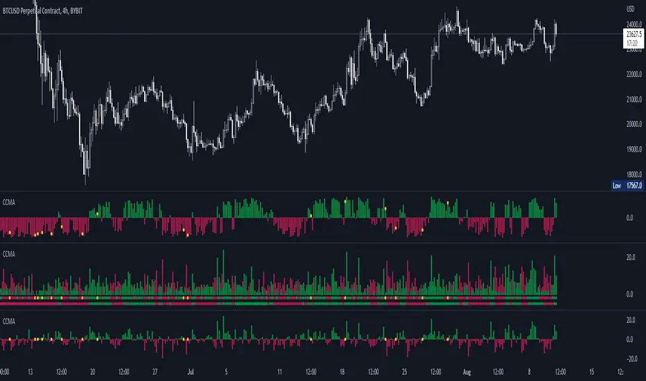
Trade System Crypto InvestidorTrade System created to facilitate the visualization of crossing and extensions of the movements with Bollinger bands.
Composed by:
Moving Averages of 21, 50, 100 and 200.
Exponential Moving Averages: 17,34,72,144, 200 and 610.
Bollinger bands with standard deviation 2 and 3.
How it works?
The indicators work together, however there are some important cross-averages that need to be identified.
- Crossing the MA21 with 50, 100 and 200 up or down will dictate an up or down trend.
- MA200 and EMA200 are excellent indicators of resistance and support zone, if the price is above these averages it will be a great support, if the price is below these averages it will indicate strong resistance.
- Another important crossover refers to exponential moving averages of 17 to 72 indicates a possible start of a trend
- The crossing of the exponential moving average of 34 with 144 will confirm the crossing mentioned above.
- In addition, the exponential moving average of 610 used by Bo Williams is an excellent reference for dictating an upward or downward trend, if the price is above it it will possibly confirm an upward trend and the downside.
- To conclude we have bollinger bands with standard deviation 2 and 3, they help to identify the maximum movements.

Moving Average Heatmap Visualization7 different types of moving averages (5 different lengths of each) compared to a base moving average. Base moving average can be configured to be a slew of different types of moving averages (credit to @mortdiggiddy for the code) and have a custom length.
Red = base moving average is over other moving average (bearish)
Green = base moving average is under other moving average (bullish)
lengths for the different MAs are just fibonacci numbers due to lack of creativity.
First 5 moving averages are Simple moving average the next 5 are Exponential moving averages and after that it is weighted moving averages, volume weighted moving average (VWAP), Exponential volume weighted moving average (thanks again @mortdiggiddy ), hull moving averages and lastly zero lag moving averages.
The indicator might lag your chart out a bit so be ready for that.
Have fun!
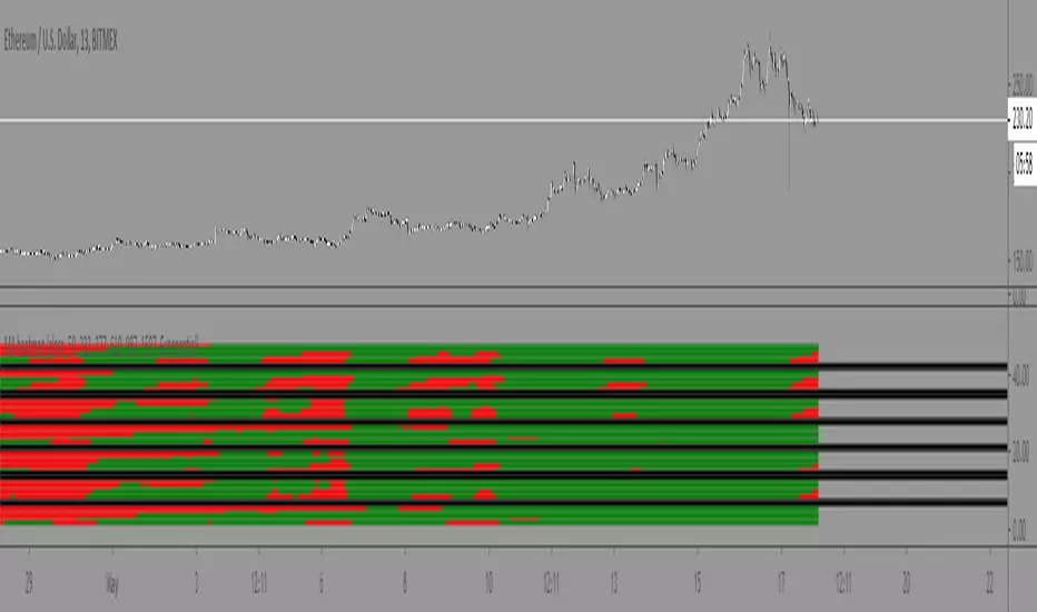
Script_Algo - High Low Range MA Crossover Strategy🎯 Core Concept
This strategy uses modified moving averages crossover, built on maximum and minimum prices, to determine entry and exit points in the market. A key advantage of this strategy is that it avoids most false signals in trendless conditions, which is characteristic of traditional moving average crossover strategies. This makes it possible to improve the risk/reward ratio and, consequently, the strategy's profitability.
📊 How the Strategy Works
Main Mechanism
The strategy builds 4 moving averages:
Two senior MAs (on high and low) with a longer period
Two junior MAs (on high and low) with a shorter period
Buy signal 🟢: when the junior MA of lows crosses above the senior MA of highs
Sell signal 🔴: when the junior MA of highs crosses below the senior MA of lows
As seen on the chart, it was potentially possible to make 9X on the WIFUSDT cryptocurrency pair in just a year and a half. However, be careful—such results may not necessarily be repeated in the future.
Special Feature
Position closing priority ❗: if an opposite signal arrives while a position is open, the strategy first closes the current position and only then opens a new one
⚙️ Indicator Settings
Available Moving Average Types
EMA - Exponential MA
SMA - Simple MA
SSMA - Smoothed MA
WMA - Weighted MA
VWMA - Volume Weighted MA
RMA - Adaptive MA
DEMA - Double EMA
TEMA - Triple EMA
Adjustable Parameters
Senior MA Length - period for long-term moving averages
Junior MA Length - period for short-term moving averages
✅ Advantages of the Strategy
🛡️ False Signal Protection - using two pairs of modified MAs reduces the number of false entries
🔄 Configuration Flexibility - ability to choose MA type and calculation periods
⚡ Automatic Switching - the strategy automatically closes the current position when receiving an opposite signal
📈 Visual Clarity - all MAs are displayed on the chart in different colors
⚠️ Disadvantages and Risks
📉 Signal Lag - like all MA-based strategies, it may provide delayed signals during sharp movements
🔁 Frequent Switching - in sideways markets, it may lead to multiple consecutive position openings/closings
📊 Requires Optimization - optimal parameters need to be selected for different instruments and timeframes
💡 Usage Recommendations
Backtest - test the strategy's performance on historical data
Optimize Parameters - select MA periods suitable for the specific trading instrument
Use Filters - add additional filters to confirm signals
Manage Risks - always use stop-loss and take-profit orders.
You can safely connect to the exchange via webhook and enjoy trading.
Good luck and profits to everyone!!
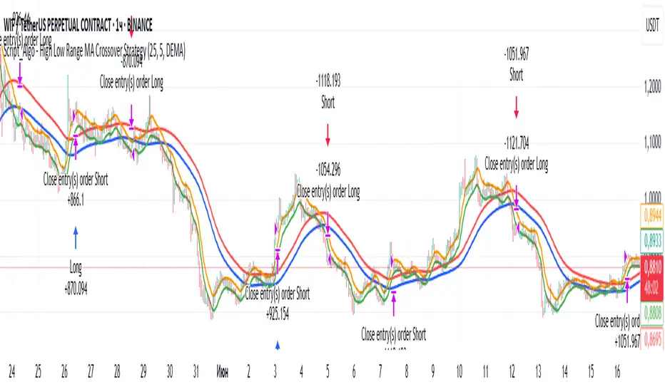
Volume MAs Oscillator | Lyro RSVolume MAs Oscillator | Lyro RS
Overview
The Volume MAs Oscillator is a powerful volume‑adjusted momentum tool that combines custom‑weighted moving averages on volume‑weighted price with smoothed deviation bands. It offers dynamic insights into trend direction, overbought/oversold conditions, and relative valuation — all within a single indicator
Key Features
Volume‑Adjusted Moving Averages: Moving averages can be volume‑weighted using the following formula: a moving average of (Price × Volume) divided by a moving average of Volume. This formula is applied across more than 14 different moving averages; however, it is not used with the VWMA, as VWMA is inherently a volume-weighted moving average.
Percentage Oscillator: Displays the normalized difference: (source – MA) / MA * 100, centered around zero for easy interpretation of strength and direction.
Deviation Bands: Builds upper and lower bands from standard deviation of the oscillator over a selected lookback, with distinct positive/negative multipliers and optional smoothing to reduce noise.
Inputs: Band Length, Band Smoothing, Positive Band Multiplier, Negative Band Multiplier.
Multi‑Mode Signal System:
1. Trend Mode – Colors oscillator according to breaks above (bullish) or below (bearish) respective bands.
2. Reversion Mode – Inverses color logic: signals overextensions beyond bands as reversion opportunities, greys inside the bands.
3. Valuation Mode – Applies a gradient color scale (UpC ⇄ DnC) to reflect relative valuation strength.
Customizable Visuals: Select from 5 pre‑set palettes—Classic, Mystic, Major Themes, Accented, Royal—or define your own custom bullish/bearish colors.
Chart enhancements include color‑coded oscillator line, deviation bands, glow‑effect midline at zero, background shading and candlestick/bar coloring aligned to signal mode.
Built‑In Signals: Automatically plots ▲ oversold and ▼ overbought markers upon crosses of lower/upper bands (in trend or reversion modes), enhancing signal clarity.
How It Works
MA Calculation – Applies the selected MA type to price × volume (normalized by MA of volume) or direct VWMA.
Oscillator Output – Calculates the % difference of source vs. derived MA.
Band Construction – Computes rolling standard deviation; applies user‑defined multipliers; smooths bands with exponential blending.
Mode-Dependent Coloring & Signals –
• Trend: Highlights strength trends via band cross coloring.
• Reversion: Flags extremes beyond bands as potential pullbacks.
• Valuation: Uses gradient to reflect oscillator’s position relative to recent range.
Signal Markers – Deploys arrows and color rules to flag overbought (▼) or oversold (▲) conditions when bands are breached.
Practical Use
Trend Confirmation – In Trend Mode, use upward price_diff cross above upper band as bullish; downward cross below lower band as bearish.
Mean Reversion – In Reversion Mode, fading extremes beyond bands may precede a retracement.
Relative Valuation – Valuation Mode shines when assessing how extended price_diff is, with gradient colors indicating valuation zones.
Bars/candles color‑coded to oscillator state boosts clarity of market tone and allows for rapid visual scanning.
Customization
Adjust MA type/length to tune responsiveness vs. smoothing.
Configure band settings for volatility sensitivity.
Toggle between signal modes for trend-following or reversion strategies.
Stylish visuals: pick or customize color schemes to match your chart setup.
⚠️Disclaimer
This indicator is a tool for technical analysis and does not provide guaranteed results. It should be used in conjunction with other analysis methods and proper risk management practices. The creators of this indicator are not responsible for any financial decisions made based on its signals.

SuperTrend MTF Pro [Cometreon]The SuperTrend MTF Pro takes the classic SuperTrend to a whole new level of customization and accuracy. Unlike the standard version, this indicator allows you to select different moving averages, apply it to various chart types, and fine-tune every key parameter.
If you're looking for an advanced, non-repainting, and highly configurable SuperTrend, this is the right choice for you.
🔷 New Features and Improvements
🟩 Multi-MA SuperTrend
Now you can customize the SuperTrend calculation by choosing from 15 different moving averages:
SMA (Simple Moving Average)
EMA (Exponential Moving Average)
WMA (Weighted Moving Average)
RMA (Smoothed Moving Average)
HMA (Hull Moving Average)
JMA (Jurik Moving Average)
DEMA (Double Exponential Moving Average)
TEMA (Triple Exponential Moving Average)
LSMA (Least Squares Moving Average)
VWMA (Volume-Weighted Moving Average)
SMMA (Smoothed Moving Average)
KAMA (Kaufman’s Adaptive Moving Average)
ALMA (Arnaud Legoux Moving Average)
FRAMA (Fractal Adaptive Moving Average)
VIDYA (Variable Index Dynamic Average)
🟩 Multiple Chart Types
You're no longer limited to candlestick charts! Now you can use SuperTrend with different chart formats, including:
Heikin Ashi
Renko
Kagi
Line Break
Point & Figure
🟩 Customizable Timeframe
Now you can adjust the SuperTrend timeframe without repainting issues, avoiding signal distortions.
🔷 Technical Details and Customizable Inputs
SuperTrend offers multiple customization options to fit any trading strategy:
1️⃣ ATR Period – Defines the ATR length, affecting the indicator’s sensitivity.
2️⃣ Source – Selects the price value used for calculations (Close, HL2, Open, etc.).
3️⃣ ATR Mult – Multiplies the ATR to determine band distance. Higher values reduce false signals, lower values make it more reactive.
4️⃣ Change ATR Calculation Method – When enabled, uses the default ATR method; when disabled, allows selecting another Moving Average with "Use Different Type".
5️⃣ Source Break – Defines the price source for trend changes (Close for more stability, High/Low for more reactivity).
6️⃣ Use Different Type – Allows selecting an alternative Moving Average for ATR calculation if "Change ATR Calculation Method" is disabled.
7️⃣ SuperTrend Type – Advanced options for specific MAs (JMA, ALMA, FRAMA, VIDYA), with dedicated parameters like Phase, Sigma, and Offset for optimized responsiveness.
8️⃣ Ticker Settings – Customize parameters for special chart types such as Renko, Heikin Ashi, Kagi, Line Break, and Point & Figure, adjusting reversal, number of lines, and ATR length.
9️⃣ Timeframe – Enables using SuperTrend on a higher timeframe.
🔟 Wait for Timeframe Closes -
✅ Enabled – Prevents multiple signals, useful for precise alerts.
❌ Disabled – Displays SuperTrend smoothly without interruptions.
🔷 How to Use SuperTrend MTF Pro
🔍 Identifying Trends
SuperTrend follows the ongoing trend and provides clear visual signals:
When the price is above the line, the trend is bullish.
When the price is below the line, the trend is bearish.
📈 Interpreting Signals
Line color and position change → Possible trend reversal
Bounce off the line → Potential trend continuation
Strong breakout of the line → Possible reversal
🛠 Integration with Other Tools
RSI or MACD to filter false signals
Moving Averages to confirm trend direction
Support and Resistance to improve entry points
☄️ If you find this indicator useful, leave a Boost to support its development!
Every feedback helps to continuously improve the tool, offering an even more effective trading experience. Share your thoughts in the comments! 🚀🔥
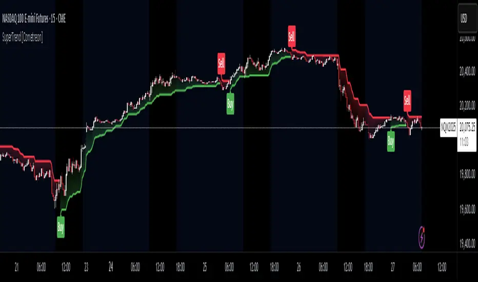
SASDv2rSensitive Altcoin Season Detector V2
This Pine Script™ code, titled "SASDv2r" (Sensitive Altcoin Season Detector version 2 revised), is designed for cryptocurrency trading analysis on the TradingView platform and tailored for those interested in tracking when altcoins might be outperforming Bitcoin, potentially indicating a market shift towards altcoins.
Feel free to use and modify. If you made it better, please let me know. Intention was to help the community with a tool for retail traders have no access to advanced, MV indicators. Solution uses classic TA only.
Use it witl TOTAL3/BTC indicator.
Please check: it gave signal just before last alt season % rose more than 250%.
Market Cap Data Fetching: The script fetches market capitalization data for Bitcoin, Ethereum, and all other altcoins (excluding Bitcoin and Ethereum) using request.security function.
Altcoin to Bitcoin Ratio: It calculates the ratio of total market cap of altcoins to Bitcoin's market cap (altToBtcRatio), which is central to identifying an "altcoin season."
Moving Averages: Several moving averages are computed for different time frames (50-day SMA, 200-day SMA, 20-day SMA, and 10-day EMA) to analyze trends in the altcoin to Bitcoin ratio.
Momentum Indicators: The script uses RSI (Relative Strength Index) and MACD (Moving Average Convergence Divergence) to gauge momentum and potential reversal points in the market.
Custom Indicators: It includes Volume Weighted Moving Average (VWMA) and a custom momentum indicator (altMomentum and altMomentumAvg) to provide additional insights into market movements.
Volatility Measurement: Bollinger Bands are calculated to assess volatility in the altcoin to Bitcoin ratio, which helps identify periods of high or low market activity.
Visual Analysis: Various plots are added to the chart for visual interpretation, including the altcoin to Bitcoin ratio, different moving averages, and Bollinger Bands.
Alt Season Detection: The script defines conditions for detecting when an "altcoin season" might be starting, based on crossovers of moving averages, RSI levels, MACD signals, and other custom criteria.
Performance Tracking: After signaling an alt season, the script evaluates the performance over the next 30 days by checking if there's been an increase in the altcoin to Bitcoin ratio, adding labels for positive or negative trends.(this one is in progress). Logic still gives false signals and aim is to identify failed signals.
Visual Signals: Labels are placed on the chart to visually indicate the beginning of a potential alt season or the performance outcome after a signal, aiding traders in making informed decisions.

2 MA Simplified Sideways Candle ColorsHow to Use the Indicator: A Simple Guide
This custom indicator colors candlesticks to help you quickly identify market conditions based on two moving averages (9-period and 21-period). Here’s how to get started:
Add the Indicator to Your Chart:
Copy the provided Pine Script code.
Open TradingView and navigate to the Pine Editor.
Paste the code into a new script, save it, and then add the indicator to your chart.
Understand the Candlestick Colors:
Green Candles (Bullish):
Indicates a bullish market when the price is above the 9-period SMA and the 9 SMA is above the 21 SMA.
Red Candles (Bearish):
Indicates a bearish market when the price is below the 21-period SMA and the 9 SMA is below the 21 SMA.
Yellow Candles (Sideways):
Indicates a sideways (neutral) market when:
Condition 1: Price is below the 9 SMA but above the 21 SMA, with the 9 SMA above the 21 SMA, or
Condition 2: The 9 SMA is below the 21 SMA, and the price lies between them.
White Candles (No Clear Signal):
Used when none of the above conditions apply.
Interpreting the Signals:
When you see green candles, the market is showing bullish momentum.
When you see red candles, bearish pressure is dominant.
Yellow candles suggest the market is moving sideways without a strong trend.
White candles mean that none of the specific conditions (bullish, bearish, or sideways) are currently met.
Chart Reference:
The script also plots two moving averages on your chart (a blue line for the 9-period SMA and an orange line for the 21-period SMA). These lines help visualize how price interacts with these averages.
Using the Indicator in Practice:
Once added to your chart, monitor the color of the candlesticks:
Green signals may be opportunities to consider long positions.
Red signals may indicate a good time to consider short positions or tighten stops.
Yellow signals suggest caution as the market isn’t trending strongly.
White candles indicate no strong signal, so it might be a period of consolidation or indecision.
This simple visual cue system allows you to quickly assess market sentiment and make more informed trading decisions based on the relationship between price and the two moving averages.

[blackcat] L1 Simple Dual Channel Breakout█ OVERVIEW
The script " L1 Simple Dual Channel Breakout" is an indicator designed to plot dual channel breakout bands and their long-term EMAs on a chart. It calculates short-term and long-term moving averages and deviations to establish upper, lower, and middle bands, which traders can use to identify potential breakout opportunities.
█ LOGICAL FRAMEWORK
Structure:
The script is structured into several main sections:
• Input Parameters: The script does not explicitly define input parameters for the user to adjust, but it uses default values for short_term_length (5) and long_term_length (181).
• Calculations: The calculate_dual_channel_breakout function performs the core calculations, including the blast condition, typical price, short-term and long-term moving averages, and dynamic moving averages.
• Plotting: The script plots the short-term bands (upper, lower, and middle) and their long-term EMAs. It also plots conditional line breaks when the short-term bands cross the long-term EMAs.
Flow of Data and Logic:
1 — The script starts by defining the calculate_dual_channel_breakout function.
2 — Inside the function, it calculates various moving averages and deviations based on the input prices and lengths.
3 — The function returns the calculated bands and EMAs.
4 — The script then calls this function with predefined lengths and plots the resulting bands and EMAs on the chart.
5 — Conditional plots are added to highlight breakouts when the short-term bands cross the long-term EMAs.
█ CUSTOM FUNCTIONS
The script defines one custom function:
• calculate_dual_channel_breakout(close_price, high_price, low_price, short_term_length, long_term_length): This function calculates the short-term and long-term bands and EMAs. It takes five parameters: close_price, high_price, low_price, short_term_length, and long_term_length. It returns an array containing the upper band, lower band, middle band, long-term upper EMA, long-term lower EMA, and long-term middle EMA.
█ KEY POINTS AND TECHNIQUES
• Typical Price Calculation: The script uses a modified typical price calculation (2 * close_price + high_price + low_price) / 4 instead of the standard (high_price + low_price + close_price) / 3.
• Short-term and Long-term Bands: The script calculates short-term bands using a simple moving average (SMA) of the typical price and long-term bands using a relative moving average (RMA) of the close price.
• Conditional Plotting: The script uses conditional plotting to highlight breakouts when the short-term bands cross the long-term EMAs, enhancing visual identification of trading signals.
• EMA for Long-term Trends: The use of Exponential Moving Averages (EMAs) for long-term bands helps in smoothing out short-term fluctuations and focusing on long-term trends.
█ EXTENDED KNOWLEDGE AND APPLICATIONS
• Modifications: Users can add input parameters to allow customization of short_term_length and long_term_length, making the indicator more flexible.
• Enhancements: The script could be extended to include alerts for breakout conditions, providing traders with real-time notifications.
• Alternative Bands: Users might experiment with different types of moving averages (e.g., WMA, HMA) for the short-term and long-term bands to see if they yield better results.
• Additional Indicators: Combining this indicator with other technical indicators (e.g., RSI, MACD) could provide a more comprehensive trading strategy.
• Backtesting: Users can backtest the strategy using Pine Script's strategy functions to evaluate its performance over historical data.

UDC - Local TrendsUDC - Local Trends Indicator
Overview:
The UDC - Local Trends Indicator combines multiple moving averages to provide a clear visualization of both local and high timeframe (HTF) trends. This indicator helps traders make informed decisions by highlighting key moving averages and trend zones, making it easier to determine whether the current trend is likely to continue or reverse.
Features:
Local Trend Zone: Displays the range between the 13 and 34 EMAs, with an average line in the middle. This zone is plotted close to the price candles, offering a clear visual guide for the immediate trend on the timeframe you’re viewing.
Usage: Observe the strength of the local trend within this zone. Breaks from this zone may indicate potential moves toward the 200 moving averages, providing early signals for trend continuation or potential reversals.
Current Trend Indicators:
Tracks the broader trend using the 200 EMA and 200 SMA on the active timeframe. Choose a timeframe where these trend lines hold significance and use them alongside support and resistance for precise entries and exits.
Cross-Timeframe Trend Reference:
On all sub-daily timeframes, the daily 200 moving average is overlaid, ensuring this essential trend line is visible even on shorter timeframes, like 4H, where reclaims or rejections of the daily 200 can signal strong trading setups.
The weekly 50 moving average, a critical HTF trend line, is also displayed consistently, guiding higher timeframe swing trade setups.
Trading Strategy:
Local Timeframe Trading:
Monitor the 200 moving averages in your active timeframe to identify bounces or breakdowns. If the local trend zone (13-34 EMA range) is lost, expect a possible pullback to the 200 moving averages, offering a chance for re-entry or confirmation of trend reversal.
High Timeframe Trading (HTF):
For swing trades, observe the daily 200 and weekly 50 moving averages. Reclaiming these lines often triggers long setups, while losing them may signal further downside until they’re regained.
This indicator offers a powerful combination of localized trend tracking and high timeframe support, enabling traders to align their entries with both immediate and overarching market

MTF EHMA & HMA Insights [FibonacciFlux]MTF EHMA & HMA Insights
Overview
The Multi-Timeframe EHMA, HMA, and Midline with Fill script is a powerful technical analysis tool designed for traders seeking to enhance their market insights and decision-making processes. By integrating two advanced moving averages—Exponential Hull Moving Average (EHMA) and Hull Moving Average (HMA)—along with a dynamic midline, this indicator provides a comprehensive view of market trends across multiple timeframes.
Key Features
1. Dual Moving Averages
- Exponential Hull Moving Average (EHMA) :
- Offers a rapid response to price changes, making it particularly useful for identifying short-term trends.
- Utilizes a unique calculation method that reduces lag, allowing traders to react quickly to market movements.
- Hull Moving Average (HMA) :
- Known for its smoothness and ability to filter out noise, the HMA presents a clear picture of the underlying trend.
- The HMA is specifically designed to achieve a balance between responsiveness and smoothness, enabling traders to make informed decisions.
2. Midline Calculation
- Dynamic Midline (m) :
- The midline is calculated as the average of EHMA and HMA, providing a neutral reference point for evaluating price movements.
- It visually represents market sentiment; a rising midline suggests bullish conditions, while a declining midline indicates bearish trends.
3. Visual Components
- Fill Areas :
- Color-coded fills between the EHMA and HMA enhance visual clarity by indicating the relative position of these moving averages.
- The fill color dynamically changes based on the relationship between the two averages (green for EHMA below HMA and red for EHMA above HMA), allowing traders to quickly assess market conditions.
4. Signal Generation and Alerts
- Buy/Sell Signals :
- The indicator generates buy signals when the midline crosses above its previous value, indicating a potential upward trend.
- Conversely, sell signals are triggered when the midline crosses below its previous value, suggesting a possible downward movement.
- Alert Conditions :
- Built-in alerts notify traders in real-time when significant changes occur, allowing them to act swiftly on potential trading opportunities.
- Customizable alert messages ensure traders receive relevant information tailored to their strategies.
Technical Details
Input Parameters
- Timeframe Settings :
- Traders can customize the timeframes for both EHMA and HMA, enabling them to adapt the indicator to different trading styles and market conditions.
- Length Settings :
- Adjustable lengths for both moving averages impact their sensitivity, allowing traders to optimize their performance based on volatility and market dynamics.
Plotting and Visualization
- Plotting :
- The script plots the EHMA, HMA, and midline directly on the chart for easy visualization.
- Signal labels (BUY and SELL) are displayed prominently, helping traders to identify potential entry and exit points without ambiguity.
Benefits
1. Clarity and Insight
- The combination of EHMA, HMA, and midline provides a clear and concise visual representation of market trends, aiding traders in making informed decisions.
2. Flexibility
- Customizable parameters allow traders to tailor the indicator to their specific needs, making it suitable for various market conditions and trading styles.
3. Efficiency
- Real-time alerts and visual signals minimize response times, enabling traders to capitalize on opportunities as they arise.
4. Enhanced Trading Conditions
- When utilizing the Fibonacci number 144 on a daily chart, the indicator facilitates optimal trading conditions:
- "The entry was made before the bubble began, using 144 as the Fibonacci variable."
- "The exit occurred right before the bubble burst, or alternatively, a short position was initiated."
- "When the next bubble started, a long entry was made again."
- "Despite some lag, the position was exited and a long entry was made."
- "The exit or short entry took place at the second double top peak."
- "A short position was already established before the double top formation occurred."
- On a 4-hour chart, traders can effectively set stop losses at HMA levels, achieving a risk-reward ratio between 4 and 8.
- Additionally, analyzing the 15-minute chart with a multi-timeframe approach allows for more precise entry points.
Conclusion
The Multi-Timeframe EHMA, HMA, and Midline with Fill script is a robust tool for traders looking to enhance their technical analysis capabilities. By combining multiple moving averages with a dynamic midline and alert system, this indicator offers a comprehensive approach to understanding market trends. Its flexibility, clarity, and efficiency make it an invaluable asset for both novice and experienced traders alike.
Important Note
As with any trading tool, it is crucial to conduct thorough analysis and risk management when using this indicator. Past performance does not guarantee future results, and traders should always be prepared for potential market fluctuations.

Deviation Adjusted MA Overview
The Deviation Adjusted MA is a custom indicator that enhances traditional moving average techniques by introducing a volatility-based adjustment. This adjustment is implemented by incorporating the standard deviation of price data, making the moving average more adaptive to market conditions. The key feature is the combination of a customizable moving average (MA) type and the application of deviation percentage to modify its responsiveness. Additionally, a smoothing layer is applied to reduce noise, improving signal clarity.
Key Components
Customizable Moving Averages
The script allows the user to select from four different types of moving averages:
Simple Moving Average (SMA): A basic average of the closing prices over a specified period.
Exponential Moving Average (EMA): Gives more weight to recent prices, making it more responsive to recent price changes.
Weighted Moving Average (WMA): Weights prices differently, favoring more recent ones but in a linear progression.
Volume-Weighted Moving Average (VWMA): Adjusts the average by trading volume, placing more weight on high-volume periods.
Standard Deviation Calculation
The script calculates the standard deviation of the closing prices over the selected maLength period.
Standard deviation measures the dispersion or volatility of price movements, giving a sense of market volatility.
Deviation Percentage and Adjustment
Deviation Percentage is calculated by dividing the standard deviation by the base moving average and multiplying by 100 to express it as a percentage.
The base moving average is adjusted by this deviation percentage, making the indicator responsive to changes in volatility. The result is a more dynamic moving average that adapts to market conditions.
The parameter devMultiplier is available to scale this adjustment, allowing further fine-tuning of sensitivity.
Smoothing the Adjusted Moving Average
After adjusting the moving average based on deviation, the script applies an additional Exponential Moving Average (EMA) with a length defined by the smoothingLength input.
This EMA serves as a smoothing filter to reduce the noise that could arise from the raw adjustments of the moving average. The smoothing makes trend recognition more consistent and removes short-term fluctuations that could otherwise distort the signal.
Use cases
The Deviation Adjusted MA indicator serves as a dynamic alternative to traditional moving averages by adjusting its sensitivity based on volatility. The script offers extensive customization options through the selection of moving average type and the parameters controlling smoothing and deviation adjustments.
By applying these adjustments and smoothing, the script enables users to better track trends and price movements, while providing a visual cue for changes in market sentiment.
