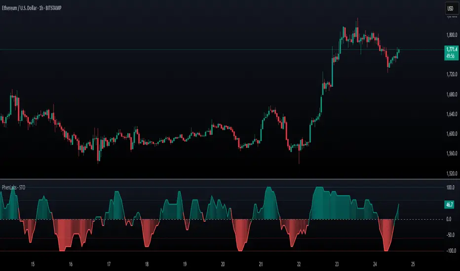
SynchroTrend Oscillator (STO) [PhenLabs]📊 SynchroTrend Oscillator
Version: PineScript™ v5
📌 Description
The SynchroTrend Oscillator (STO) is a multi-timeframe synchronization tool that combines trend information from three distinct timeframes into a single, easy-to-interpret oscillator ranging from -100 to +100.
This indicator solves the common problem of having to analyze multiple timeframe charts separately by consolidating trend direction and strength across different time horizons. The STO helps traders identify when markets are truly synchronized across timeframes, potentially indicating stronger trend conditions and higher probability trading opportunities.
Using either Moving Average crossovers or RSI analysis as the trend definition metric, the STO provides a comprehensive view of market structure that adapts to various trading strategies and market conditions.
🚀 Points of Innovation
Triple-timeframe synchronization in a single view eliminates chart switching
Dual trend detection methods (MA vs Price or RSI) for flexibility across different markets
Dynamic color intensity that automatically increases with signal strength
Scaled oscillator format (-100 to +100) for intuitive trend strength interpretation
Customizable signal thresholds to match your risk tolerance and trading style
Visual alerts when markets reach full synchronization states
🔧 Core Components
Trend Scoring System: Calculates a binary score (+1, -1, or 0) for each timeframe based on selected metrics, providing clear trend direction
Multi-Timeframe Synchronization: Combines and scales trend scores from all three timeframes into a single oscillator
Dynamic Visualization: Adjusts color transparency based on signal strength, creating an intuitive visual guide
Threshold System: Provides customizable levels for identifying potentially significant trading opportunities
🔥 Key Features
Triple Timeframe Analysis: Synchronizes three user-defined timeframes (default: 60min, 15min, 5min) into one view
Dual Trend Detection Methods: Choose between Moving Average vs Price or RSI-based trend determination
Adjustable Signal Smoothing: Apply EMA, SMA, or no smoothing to the oscillator output for your preferred signal responsiveness
Dynamic Color Intensity: Colors become more vibrant as signal strength increases, helping identify strongest setups
Customizable Thresholds: Set your own buy/sell threshold levels to match your trading strategy
Comprehensive Alerts: Six different alert conditions for crossing thresholds, zero line, and full synchronization states
🎨 Visualization
Oscillator Line: The main line showing the synchronized trend value from -100 to +100
Dynamic Fill: Area between oscillator and zero line changes transparency based on signal strength
Threshold Lines: Optional dotted lines indicating buy/sell thresholds for visual reference
Color Coding: Green for bullish synchronization, red for bearish synchronization
📖 Usage Guidelines
Timeframe Settings
Timeframe 1: Default: 60 (1 hour) - Primary higher timeframe for trend definition
Timeframe 2: Default: 15 (15 minutes) - Intermediate timeframe for trend definition
Timeframe 3: Default: 5 (5 minutes) - Lower timeframe for trend definition
Trend Calculation Settings
Trend Definition Metric: Default: “MA vs Price” - Method used to determine trend on each timeframe
MA Type: Default: EMA - Moving Average type when using MA vs Price method
MA Length: Default: 21 - Moving Average period when using MA vs Price method
RSI Length: Default: 14 - RSI period when using RSI method
RSI Source: Default: close - Price data source for RSI calculation
Oscillator Settings
Smoothing Type: Default: SMA - Applies smoothing to the final oscillator
Smoothing Length: Default: 5 - Period for the smoothing function
Visual & Threshold Settings
Up/Down Colors: Customize colors for bullish and bearish signals
Transparency Range: Control how transparency changes with signal strength
Line Width: Adjust oscillator line thickness
Buy/Sell Thresholds: Set levels for potential entry/exit signals
✅ Best Use Cases
Trend confirmation across multiple timeframes
Finding high-probability entry points when all timeframes align
Early detection of potential trend reversals
Filtering trade signals from other indicators
Market structure analysis
Identifying potential divergences between timeframes
⚠️ Limitations
Like all indicators, can produce false signals during choppy or ranging markets
Works best in trending market conditions
Should not be used in isolation for trading decisions
Past performance is not indicative of future results
May require different settings for different markets or instruments
💡 What Makes This Unique
Combines three timeframes in a single visualization without requiring multiple chart windows
Dynamic transparency feature that automatically emphasizes stronger signals
Flexible trend definition methods suitable for different market conditions
Visual system that makes multi-timeframe analysis intuitive and accessible
🔬 How It Works
1. Trend Evaluation:
For each timeframe, the indicator calculates a trend score (+1, -1, or 0) using either:
MA vs Price: Comparing close price to a moving average
RSI: Determining if RSI is above or below 50
2. Score Aggregation:
The three trend scores are combined and then scaled to a range of -100 to +100
A value of +100 indicates all timeframes show bullish conditions
A value of -100 indicates all timeframes show bearish conditions
Values in between indicate varying degrees of alignment
3. Signal Processing:
The raw oscillator value can be smoothed using EMA, SMA, or left unsmoothed
The final value determines line color, fill color, and transparency settings
Threshold levels are applied to identify potential trading opportunities
💡 Note:
The SynchroTrend Oscillator is most effective when used as part of a comprehensive trading strategy that includes proper risk management techniques. For best results, consider using the oscillator in conjunction with support/resistance levels, price action analysis, and other complementary indicators that align with your trading style.
Tìm kiếm tập lệnh với "oscillator"
Realized Price Oscillator [InvestorUnknown]Overview
The Realized Price Oscillator is a fundamental analysis tool designed to assess Bitcoin's price dynamics relative to its realized price. The indicator calculates various metrics using data from the realized market capitalization and total supply. It applies normalization techniques to scale values within a specified range, helping investors identify overbought or oversold conditions over the long time horizon. The oscillator also features DCA-based signals to assist in strategic market entry and exit.
Key Features
1. Normalization and Scaling:
The indicator scales values using a limit that can be adjusted for decimal precision (Limit). It allows for both positive and negative values, providing flexibility in analysis.
Decay functionality is included to progressively reduce the extreme values over time, ensuring recent data impacts the oscillator more than older data.
f_rescale(float value, float min, float max, float limit, bool negatives) =>
((limit * (negatives ? 2 : 1)) * (value - min) / (max - min)) - (negatives ? limit : 0)
2. Realized Price Oscillator Calculation:
Realized Price Oscillator is computed using logarithmic differences between the open, high, low, and close prices and the realized price. This helps in identifying how the current market price compares with the average cost basis of the Bitcoin supply.
f_realized_price_oscillator(float realized_price) =>
rpo_o = math.log(open / realized_price)
rpo_h = math.log(high / realized_price)
rpo_l = math.log(low / realized_price)
rpo_c = math.log(close / realized_price)
3. Oscillator Normalization:
The normalized oscillator calculates the range between the maximum and minimum values over time. It adjusts the oscillator values based on these bounds, considering a decay factor. This normalized range assists in consistent signal generation.
normalized_oscillator(float x, float b) =>
float oscillator = b
var float min = na
var float max = na
if (oscillator > max or na(max)) and time >= normalization_start_date
max := oscillator
if (min > oscillator or na(min)) and time >= normalization_start_date
min := oscillator
if time >= normalization_start_date
max := max * decay
min := min * decay
normalized_oscillator = f_rescale(x, min, max, lim, neg)
4. Dollar-Cost Averaging (DCA) Signals:
DCA-based signals are generated using user-defined thresholds (DCA IN and DCA OUT). The oscillator triggers buy signals when the normalized low value falls below the DCA IN threshold and sell signals when the normalized high value exceeds the DCA OUT threshold.
5. Visual Representation:
The indicator plots candlestick representations of the normalized Realized Price Oscillator values (open, high, low, close) over time, starting from a specified date (plot_start_date).
Colors are dynamically adjusted using a gradient to represent the state of the oscillator, ranging from green (buy zone) to red (sell zone). Background and bar colors also change based on DCA conditions.
How It Works
Data Sourcing: Realized price data is sourced using Bitcoin’s realized market cap (BTC_MARKETCAPREAL) and total supply (BTC_SUPPLY).
Realized Price Oscillator Metrics: Logarithmic differences between price and realized price are computed to generate Realized Price Oscillator values for open, high, low, and close.
Normalization: The indicator rescales the oscillator values based on a defined limit, adjusting for negative values if allowed. It employs a decay factor to reduce the influence of historical extremes.
Conclusion
The Realized Price Oscillator is a sophisticated tool that combines market price analysis with realized price metrics to offer a robust framework for understanding Bitcoin's valuation. By leveraging normalization techniques and DCA thresholds, it provides actionable insights for long-term investing strategies.

Bitcoin Power Law Oscillator [InvestorUnknown]The Bitcoin Power Law Oscillator is a specialized tool designed for long-term mean-reversion analysis of Bitcoin's price relative to a theoretical midline derived from the Bitcoin Power Law model (made by capriole_charles). This oscillator helps investors identify whether Bitcoin is currently overbought, oversold, or near its fair value according to this mathematical model.
Key Features:
Power Law Model Integration: The oscillator is based on the midline of the Bitcoin Power Law, which is calculated using regression coefficients (A and B) applied to the logarithm of the number of days since Bitcoin’s inception. This midline represents a theoretical fair value for Bitcoin over time.
Midline Distance Calculation: The distance between Bitcoin’s current price and the Power Law midline is computed as a percentage, indicating how far above or below the price is from this theoretical value.
float a = input.float (-16.98212206, 'Regression Coef. A', group = "Power Law Settings")
float b = input.float (5.83430649, 'Regression Coef. B', group = "Power Law Settings")
normalization_start_date = timestamp(2011,1,1)
calculation_start_date = time == timestamp(2010, 7, 19, 0, 0) // First BLX Bitcoin Date
int days_since = request.security('BNC:BLX', 'D', ta.barssince(calculation_start_date))
bar() =>
= request.security('BNC:BLX', 'D', bar())
int offset = 564 // days between 2009/1/1 and "calculation_start_date"
int days = days_since + offset
float e = a + b * math.log10(days)
float y = math.pow(10, e)
float midline_distance = math.round((y / btc_close - 1.0) * 100)
Oscillator Normalization: The raw distance is converted into a normalized oscillator, which fluctuates between -1 and 1. This normalization adjusts the oscillator to account for historical extremes, making it easier to compare current conditions with past market behavior.
float oscillator = -midline_distance
var float min = na
var float max = na
if (oscillator > max or na(max)) and time >= normalization_start_date
max := oscillator
if (min > oscillator or na(min)) and time >= normalization_start_date
min := oscillator
rescale(float value, float min, float max) =>
(2 * (value - min) / (max - min)) - 1
normalized_oscillator = rescale(oscillator, min, max)
Overbought/Oversold Identification: The oscillator provides a clear visual representation, where values near 1 suggest Bitcoin is overbought, and values near -1 indicate it is oversold. This can help identify potential reversal points or areas of significant market imbalance.
Optional Moving Average: Users can overlay a moving average (either SMA or EMA) on the oscillator to smooth out short-term fluctuations and focus on longer-term trends. This is particularly useful for confirming trend reversals or persistent overbought/oversold conditions.
This indicator is particularly useful for long-term Bitcoin investors who wish to gauge the market's mean-reversion tendencies based on a well-established theoretical model. By focusing on the Power Law’s midline, users can gain insights into whether Bitcoin’s current price deviates significantly from what historical trends would suggest as a fair value.

S&P Short-Range Oscillator**SHOULD BE USED ON THE S&P 500 ONLY**
The S&P Short-Range Oscillator (SRO), inspired by the principles of Jim Cramer's oscillator, is a technical analysis tool designed to help traders identify potential buy and sell signals in the stock market, specifically for the S&P 500 index. The SRO combines several market indicators to provide a normalized measure of market sentiment, assisting traders in making informed decisions.
The SRO utilizes two simple moving averages (SMAs) of different lengths: a 5-day SMA and a 10-day SMA. It also incorporates the daily price change and market breadth (the net change of closing prices). The 5-day and 10-day SMAs are calculated based on the closing prices. The daily price change is determined by subtracting the opening price from the closing price. Market breadth is calculated as the difference between the current closing price and the previous closing price.
The raw value of the oscillator, referred to as SRO Raw, is the sum of the daily price change, the 5-day SMA, the 10-day SMA, and the market breadth. This raw value is then normalized using its mean and standard deviation over a 20-day period, ensuring that the oscillator is centered and maintains a consistent scale. Finally, the normalized value is scaled to fit within the range of -15 to 15.
When interpreting the SRO, a value below -5 indicates that the market is potentially oversold, suggesting it might be a good time to start buying stocks as the market could be poised for a rebound. Conversely, a value above 5 suggests that the market is potentially overbought. In this situation, it may be prudent to hold on to existing positions or consider selling if you have substantial gains.
The SRO is visually represented as a blue line on a chart, making it easy to track its movements. Red and green horizontal lines mark the overbought (5) and oversold (-5) levels, respectively. Additionally, the background color changes to light red when the oscillator is overbought and light green when it is oversold, providing a clear visual cue.
By incorporating the S&P Short-Range Oscillator into your trading strategy, you can gain valuable insights into market conditions and make more informed decisions about when to buy, sell, or hold your stocks. However, always consider other market factors and perform your own analysis before making any trading decisions.
The S&P Short-Range Oscillator is a powerful tool for traders looking to gain insights into market sentiment. It provides clear buy and sell signals through its combination of multiple indicators and normalization process. However, traders should be aware of its lagging nature and potential complexity, and use it in conjunction with other analysis methods for the best results.
Disclaimer
The S&P Short-Range Oscillator is for informational purposes only and should not be considered financial advice. Trading involves risk, and you should conduct your own research or consult a financial advisor before making investment decisions. The author is not responsible for any losses incurred from using this indicator. Use at your own risk.

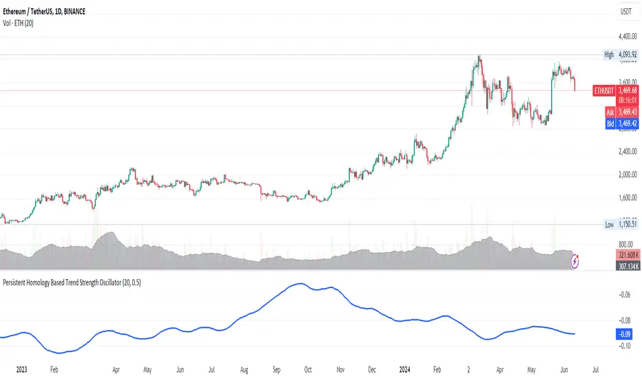
Persistent Homology Based Trend Strength OscillatorPersistent Homology Based Trend Strength Oscillator
The Persistent Homology Based Trend Strength Oscillator is a unique and powerful tool designed to measure the persistence of market trends over a specified rolling window. By applying the principles of persistent homology, this indicator provides traders with valuable insights into the strength and stability of uptrends and downtrends, helping to inform better trading decisions.
What Makes This Indicator Original?
This indicator's originality lies in its application of persistent homology , a method from topological data analysis, to financial markets. Persistent homology examines the shape and features of data across multiple scales, identifying patterns that persist as the scale changes. By adapting this concept, the oscillator tracks the persistence of uptrends and downtrends in price data, offering a novel approach to trend analysis.
Concepts Underlying the Calculations:
Persistent Homology: This method identifies features such as clusters, holes, and voids that persist as the scale changes. In the context of this indicator, it tracks the duration and stability of price trends.
Rolling Window Analysis: The oscillator uses a specified window size to calculate the average length of uptrends and downtrends, providing a dynamic view of trend persistence over time.
Threshold-Based Trend Identification: It differentiates between uptrends and downtrends based on specified thresholds for price changes, ensuring precision in trend detection.
How It Works:
The oscillator monitors consecutive changes in closing prices to identify uptrends and downtrends.
An uptrend is detected when the closing price increase exceeds a specified positive threshold.
A downtrend is detected when the closing price decrease exceeds a specified negative threshold.
The lengths of these trends are recorded and averaged over the chosen window size.
The Trend Persistence Index is calculated as the difference between the average uptrend length and the average downtrend length, providing a measure of trend persistence.
How Traders Can Use It:
Identify Trend Strength: The Trend Persistence Index offers a clear measure of the strength and stability of uptrends and downtrends. A higher value indicates stronger and more persistent uptrends, while a lower value suggests stronger and more persistent downtrends.
Spot Trend Reversals: Significant shifts in the Trend Persistence Index can signal potential trend reversals. For instance, a transition from positive to negative values might indicate a shift from an uptrend to a downtrend.
Confirm Trends: Use the Trend Persistence Index alongside other technical indicators to confirm the strength and duration of trends, enhancing the accuracy of your trading signals.
Manage Risk: Understanding trend persistence can help traders manage risk by identifying periods of high trend stability versus periods of potential volatility. This can be crucial for timing entries and exits.
Example Usage:
Default Settings: Start with the default settings to get a feel for the oscillator’s behavior. Observe how the Trend Persistence Index reacts to different market conditions.
Adjust Thresholds: Fine-tune the positive and negative thresholds based on the asset's volatility to improve trend detection accuracy.
Combine with Other Indicators: Use the Persistent Homology Based Trend Strength Oscillator in conjunction with other technical indicators such as moving averages, RSI, or MACD for a comprehensive analysis.
Backtesting: Conduct backtesting to see how the oscillator would have performed in past market conditions, helping you to refine your trading strategy.
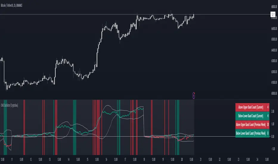
CME Gap Oscillator [CryptoSea]Introducing the CME Gap Oscillator , a pioneering tool designed to illuminate the significance of market gaps through the lens of the Chicago Mercantile Exchange (CME). By leveraging gap sizes in relation to the Average True Range (ATR), this indicator offers a unique perspective on market dynamics, particularly around the critical weekly close periods.
Key Features
Gap Measurement : At its core, the CME Oscillator quantifies the size of weekend gaps in the context of the market's volatility, using the ATR to standardize this measurement.
Dynamic Levels : Incorporating a dynamic extreme level calculation, the tool adapts to current market conditions, providing real-time insights into significant gap sizes and their implications.
Band Analysis : Through the introduction of upper and lower bands, based on standard deviations, traders can visually assess the oscillator's position relative to typical market ranges.
Enhanced Insights : A built-in table tracks the frequency of the oscillator's breaches beyond these bands within the latest CME week, offering a snapshot of recent market extremities.
Settings & Customisation
ATR-Based Measurement : Choose to measure gap sizes directly or in terms of ATR for a volatility-adjusted view.
Band Period Adjustability : Tailor the oscillator's sensitivity by modifying the band calculation period.
Dynamic Level Multipliers : Adjust the multiplier for dynamic levels to suit your analysis needs.
Visual Preferences : Customise the oscillator, bands, and table visuals, including color schemes and line styles.
In the example below, it demonstrates that the CME will want to return to the 0 value, this would be considered a reset or gap fill.
Application & Strategy
Deploy the CME Oscillator to enhance your market analysis
Market Sentiment : Gauge weekend market sentiment shifts through gap analysis, refining your strategy for the week ahead.
Volatility Insights : Use the oscillator's ATR-based measurements to understand the volatility context of gaps, aiding in risk management.
Trend Identification : Identify potential trend continuations or reversals based on the frequency and magnitude of gaps exceeding dynamic levels.
The CME Oscillator stands out as a strategic tool for traders focusing on gap analysis and volatility assessment. By offering a detailed breakdown of market gaps in relation to volatility, it empowers users with actionable insights, enabling more informed trading decisions across a range of markets and timeframes.
Normalised T3 Oscillator [BackQuant]Normalised T3 Oscillator
The Normalised T3 Oscillator is an technical indicator designed to provide traders with a refined measure of market momentum by normalizing the T3 Moving Average. This tool was developed to enhance trading decisions by smoothing price data and reducing market noise, allowing for clearer trend recognition and potential signal generation. Below is a detailed breakdown of the Normalised T3 Oscillator, its methodology, and its application in trading scenarios.
1. Conceptual Foundation and Definition of T3
The T3 Moving Average, originally proposed by Tim Tillson, is renowned for its smoothness and responsiveness, achieved through a combination of multiple Exponential Moving Averages and a volume factor. The Normalised T3 Oscillator extends this concept by normalizing these values to oscillate around a central zero line, which aids in highlighting overbought and oversold conditions.
2. Normalization Process
Normalization in this context refers to the adjustment of the T3 values to ensure that the oscillator provides a standard range of output. This is accomplished by calculating the lowest and highest values of the T3 over a user-defined period and scaling the output between -0.5 to +0.5. This process not only aids in standardizing the indicator across different securities and time frames but also enhances comparative analysis.
3. Integration of the Oscillator and Moving Average
A unique feature of the Normalised T3 Oscillator is the inclusion of a secondary smoothing mechanism via a moving average of the oscillator itself, selectable from various types such as SMA, EMA, and more. This moving average acts as a signal line, providing potential buy or sell triggers when the oscillator crosses this line, thus offering dual layers of analysis—momentum and trend confirmation.
4. Visualization and User Interaction
The indicator is designed with user interaction in mind, featuring customizable parameters such as the length of the T3, normalization period, and type of moving average used for signals. Additionally, the oscillator is plotted with a color-coded scheme that visually represents different strength levels of the market conditions, enhancing readability and quick decision-making.
5. Practical Applications and Strategy Integration
Traders can leverage the Normalised T3 Oscillator in various trading strategies, including trend following, counter-trend plays, and as a component of a broader trading system. It is particularly useful in identifying turning points in the market or confirming ongoing trends. The clear visualization and customizable nature of the oscillator facilitate its adaptation to different trading styles and market environments.
6. Advanced Features and Customization
Further enhancing its utility, the indicator includes options such as painting candles according to the trend, showing static levels for quick reference, and alerts for crossover and crossunder events, which can be integrated into automated trading systems. These features allow for a high degree of personalization, enabling traders to mold the tool according to their specific trading preferences and risk management requirements.
7. Theoretical Justification and Empirical Usage
The use of the T3 smoothing mechanism combined with normalization is theoretically sound, aiming to reduce lag and false signals often associated with traditional moving averages. The practical effectiveness of the Normalised T3 Oscillator should be validated through rigorous backtesting and adjustment of parameters to match historical market conditions and volatility.
8. Conclusion and Utility in Market Analysis
Overall, the Normalised T3 Oscillator by BackQuant stands as a sophisticated tool for market analysis, providing traders with a dynamic and adaptable approach to gauging market momentum. Its development is rooted in the understanding of technical nuances and the demand for a more stable, responsive, and customizable trading indicator.
Thus following all of the key points here are some sample backtests on the 1D Chart
Disclaimer: Backtests are based off past results, and are not indicative of the future.
INDEX:BTCUSD
INDEX:ETHUSD
BINANCE:SOLUSD

Composite Trend Oscillator [ChartPrime]CODE DUELLO:
Have you ever stopped to wonder what the underlying filters contained within complex algorithms are actually providing for you? Wouldn't it be nice to actually visually inspect for that? Those would require some kind of wild west styled quick draw duel or some comparison method as a proper 'code duello'. Then it can be determined which filter can 'draw' the quickest from it's computational holster with the least amount of lag and smoothness.
In Pine we can do so, discovering how beneficial that would be. This can be accomplished by quickly switching from one filter to another by input() back and forth, requiring visual memory. A better way could be done by placing two indicators added to the chart and then eventually placed into one indicator pane on top of each other.
By adding a filter() helper function that calls other moving average functions chosen for comparison, it can put to the test which moving average is the best drawing filter suited to our expected needs. PhiSmoother was formerly debuted and now it is utilized in a more complex environment in a multitude of ways along side other commonly utilized filters. Now, you the reader, get to judge for yourself...
FILTER VERSATILITY:
Having the capability to adjust between various smoothing methods such as PhiSmoother, TEMA, DEMA, WMA, EMA, and SMA on historical market data within the code provides an advantage. Each of these filter methods offers distinct advantages and hinderances. PhiSmoother stands out often by having superb noise rejection, while also being able to manipulate the fine-tuning of the phase or lag of the indicator, enhancing responsiveness to price movements.
The following are more well-known classic filters. TEMA (Triple Exponential Moving Average) and DEMA (Double Exponential Moving Average) offer reduced transient response times to price changes fluctuations. WMA (Weighted Moving Average) assigns more weight to recent data points, making it particularly useful for reduced lag. EMA (Exponential Moving Average) strikes a balance between responsiveness and computational efficiency, making it a popular choice. SMA (Simple Moving Average) provides a straightforward calculation based on the arithmetic mean of the data. VWMA and RMA have both been excluded for varying reasons, both being unworthy of having explanation here.
By allowing for adjustment refinements between these filter methods, traders may garner the flexibility to adapt their analysis to different market dynamics, optimizing their algorithms for improved decision-making and performance on demand.
INDICATOR INTRODUCTION:
ChartPrime's Composite Trend Oscillator operates as an oscillator based on the concept of a moving average ribbon. It utilizes up to 32 filters with progressively longer periods to assess trend direction and strength. Embedded within this indicator is an alternative view that utilizes the separation of the ribbon filaments to assess volatility. Both versions are excellent candidates for trend and momentum, both offering visualization of polarity, directional coloring, and filter crossings. Anyone who has former experience using RSI or stochastics may have ease of understanding applying this to their chart.
COMPOSITE CLUSTER MODES EXPLAINED:
In Trend Strength mode, the oscillator behavior signifies market direction and movement strength. When the oscillator is rising and above zero, the market is within a bullish phase, and visa versa. If the signal filter crosses the composite trend, this indicates a potential dynamic shift signaling a possible reversal. When the oscillator is teetering on its extremities, the market is more inclined to reverse later.
With Volatility mode, the oscillator undergoes a transformation, displaying an unbounded oscillator driven by market volatility. While it still employs the same scoring mechanism, it is now scaled according to the strength of the market move. This can aid with identification of ranging scenarios. However, one side effect is that the oscillator no longer has minimum or maximum boundaries. This can still be advantageous when considering divergences.
NOTEWORTHY SETTINGS FEATURES:
The following input settings described offer comprehensive control over the indicator's behavior and visualization.
Common Controls:
Price Source Selection - The indicator offers flexibility in choosing the price source for analysis. Traders can select from multiple options.
Composite Cluster Mode - Choose between "Trend Strength" and "Volatility" modes, providing insights into trend directionality or volatility weighting.
Cluster Filter and Length - Selects a filter for the cluster composition. This includes a length parameter adjustment.
Cluster Options:
Cluster Dispersion - Users can adjust the separation between moving averages in the cluster, influencing the sensitivity of the analysis.
Cluster Trimming - By modifying upper and lower trim parameters, traders can adjust the sensitivity of the moving averages within the cluster, enhancing its adaptability.
PostSmooth Filter and Length - Choose a filter to refine the composite cluster's post-smoothing with a length parameter adjustment.
Signal Filter and Length - Users can select a filter for the lagging signal plot, also having a length parameter adjustment.
Transition Easing - Sensitivity adjustment to influence the transition between bullish and bearish colors.
Enjoy

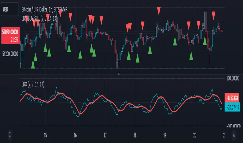
CBO (Candle Bias Oscillator)The Candle Bias Oscillator (CBO) with volume and ATR scaling is a unique technical analysis tool designed to capture market sentiment through the analysis of candlestick patterns, volume momentum, and market volatility. This indicator is built on the foundation of assessing the bias within a candlestick's body and wicks, adjusted for market volatility using the Average True Range (ATR), and further refined by comparing the Rate of Change (ROC) in volume and the adjusted bias. The culmination of these calculations results in the CBO, a smoothed oscillator that highlights potential market turning points through divergence analysis.
Key Features:
Bias Calculations: Utilizes the relationship between the candle's body and wicks to determine the market's immediate bias, offering a nuanced view beyond simple price action. Have you ever wanted to quantify exactly how bullish or bearish a particular candle or candlestick pattern is? Whether it's dojis, hammers, engulfing, gravestones, evening morning star, three soldiers etc. you don't have to memorize 50 candlestick patterns anymore.
Volatility Adjustment: Employs the ATR to adjust the bias calculation, ensuring the oscillator remains relevant across varying market conditions by accounting for volatility.
Momentum and Divergence: Measures the momentum in volume and bias through ROC calculations, identifying divergence that may signal reversals or significant price movements.
Signal Line: A smoothed version of the CBO, derived from its own values, serving as a benchmark for identifying potential crossovers and divergences.
Utility and Application:
The CBO with Divergence Scaling is developed for traders who seek a deeper understanding of market dynamics beyond price movements alone. It is particularly useful for identifying potential reversals or continuation patterns early, by highlighting divergence between market sentiment (as expressed through candlestick bias) and actual volume movements. In this way, it aligns us retail traders with institutional traders and smart money. This indicator is versatile and can be applied across various time frames and market instruments, offering value to both short-term traders and long-term investors.
How to Use:
Trend Identification: The direction and value of the CBO provide insights into the prevailing market trend. A positive oscillator value may indicate bullish sentiment, while a negative value suggests bearish sentiment.
Signal Line Crossovers: Crossovers between the CBO and its signal line can be used as potential buy or sell signals. A crossover above the signal line might indicate a buying opportunity, whereas a crossover below could suggest a selling point.
Divergence: Discrepancies between the CBO and price action (especially when confirmed by volume ROC) can highlight potential reversals.
Customization and Parameters: This script allows users to adjust several parameters, including oscillator periods, signal line periods, ATR periods, and ROC periods for divergence, to best fit their trading strategy and the characteristics of the market they are analyzing.
Conclusion:
The Custom Bias Oscillator with Divergence Scaling is a comprehensive tool designed to offer traders a multi-faceted view of market conditions, combining elements of price action, volatility, and momentum. By integrating these aspects into a single indicator, it aims to provide a more rounded and actionable insight into market trends and potential turning points.
To comply with best practices and ensure clarity regarding the informational nature of the Custom Bias Oscillator (CBO) tool, it's crucial to include a disclaimer about the non-advisory nature of the script. Here's a suitable disclaimer that you can add to the end of your script description or publication:
Disclaimer:
The Custom Bias Oscillator (CBO) with Divergence Scaling and its accompanying analysis are provided as tools for educational and informational purposes only and should not be construed as financial advice. The creator of this indicator does not guarantee any specific outcomes or profit, and all users should be aware of the risks involved in trading and investing. Users should conduct their own research and consult with a professional financial advisor before making any investment decisions. The use of this indicator is at the user's own risk, and the creator bears no responsibility for any direct or consequential loss arising from any use of this tool or the information provided herein.
Normalized Elastic Volume Oscillator (MTF)The Multi-Timeframe Normalized Elastic Volume Oscillator combines volume analysis with multiple timeframe analysis. It provides traders with valuable insights into volume dynamics across different timeframes, helping to identify trends, potential reversals, and overbought/oversold conditions.
When using the Multi-Timeframe Normalized Elastic Volume Oscillator, consider the following guidelines:
Understanding Input Parameters : The indicator offers customizable input parameters to suit your trading preferences. You can adjust the EMA length (emaLength), scaling factor (scalingFactor), volume weighting option (volumeWeighting), and select a higher timeframe for analysis (higherTF). Experiment with these parameters to optimize the indicator for your trading strategy.
Multiple Timeframe Analysis : The Multi-Timeframe Normalized Elastic Volume Oscillator allows you to analyze volume dynamics on both the current timeframe and a higher timeframe. By comparing volume behavior across different timeframes, you gain a broader perspective on market trends and the strength of volume deviations. The higher timeframe analysis provides additional confirmation and helps identify more significant market shifts.
Normalized Values : The indicator normalizes the volume deviations on both timeframes to a consistent scale between -0.25 and 0.75. This normalization makes it easier to compare and interpret the oscillator's readings across different assets and timeframes. Positive values indicate bullish volume behavior, while negative values suggest bearish volume behavior.
Interpreting the Indicator : Pay attention to the position of the Multi-Timeframe Normalized Elastic Volume Oscillator lines relative to the zero line on both timeframes. Positive values on either timeframe indicate a bullish bias, while negative values suggest a bearish bias. The distance of the oscillator from the zero line reflects the strength of the volume deviation. Extreme readings, both positive and negative, may indicate overbought or oversold conditions, potentially signaling a trend reversal or exhaustion.
Combining with Other Indicators : For more robust trading decisions, consider combining the Multi-Timeframe Normalized Elastic Volume Oscillator with other technical analysis tools. This could include trend indicators, support/resistance levels, or candlestick patterns. By incorporating multiple indicators, you gain additional confirmation and increase the reliability of your trading signals.
Remember that the Multi-Timeframe Normalized Elastic Volume Oscillator is a valuable tool, but it should not be used in isolation. Consider other factors such as price action, market context, and fundamental analysis to make well-informed trading decisions. Additionally, practice proper risk management and exercise caution when executing trades.
By utilizing the Multi-Timeframe Normalized Elastic Volume Oscillator, you gain a comprehensive view of volume dynamics across different timeframes. This knowledge can help you identify potential market trends, confirm trading signals, and improve the timing of your trades.
Take time to familiarize yourself with the indicator and conduct thorough testing on historical data. This will help you gain confidence in its effectiveness and align it with your trading strategy. With experience and continuous evaluation, you can harness the power of the Multi-Timeframe Normalized Elastic Volume Oscillator to make informed trading decisions.

Combo Backtest 123 Reversal & Rainbow Oscillator This is combo strategies for get a cumulative signal.
First strategy
This System was created from the Book "How I Tripled My Money In The
Futures Market" by Ulf Jensen, Page 183. This is reverse type of strategies.
The strategy buys at market, if close price is higher than the previous close
during 2 days and the meaning of 9-days Stochastic Slow Oscillator is lower than 50.
The strategy sells at market, if close price is lower than the previous close price
during 2 days and the meaning of 9-days Stochastic Fast Oscillator is higher than 50.
Second strategy
Ever since the people concluded that stock market price movements are not
random or chaotic, but follow specific trends that can be forecasted, they
tried to develop different tools or procedures that could help them identify
those trends. And one of those financial indicators is the Rainbow Oscillator
Indicator. The Rainbow Oscillator Indicator is relatively new, originally
introduced in 1997, and it is used to forecast the changes of trend direction.
As market prices go up and down, the oscillator appears as a direction of the
trend, but also as the safety of the market and the depth of that trend. As
the rainbow grows in width, the current trend gives signs of continuity, and
if the value of the oscillator goes beyond 80, the market becomes more and more
unstable, being prone to a sudden reversal. When prices move towards the rainbow
and the oscillator becomes more and more flat, the market tends to remain more
stable and the bandwidth decreases. Still, if the oscillator value goes below 20,
the market is again, prone to sudden reversals. The safest bandwidth value where
the market is stable is between 20 and 80, in the Rainbow Oscillator indicator value.
The depth a certain price has on a chart and into the rainbow can be used to judge
the strength of the move.
WARNING:
- For purpose educate only
- This script to change bars colors.
Bilateral Stochastic Oscillator - For The Sake Of EfficiencyIntroduction
The stochastic oscillator is a feature scaling method commonly used in technical analysis, this method is the same as the running min-max normalization method except that the stochastic oscillator is in a range of (0,100) while min-max normalization is in a range of (0,1). The stochastic oscillator in itself is efficient since it tell's us when the price reached its highest/lowest or crossed this average, however there could be ways to further develop the stochastic oscillator, this is why i propose this new indicator that aim to show all the information a classical stochastic oscillator would give with some additional features.
Min-Max Derivation
The min-max normalization of the price is calculated as follow : (price - min)/(max - min) , this calculation is efficient but there is alternates forms such as :
price - (max - min) - min/(max - min)
This alternate form is the one i chosen to make the indicator except that both range (max - min) are smoothed with a simple moving average, there are also additional modifications that you can see on the code.
The Indicator
The indicator return two main lines, in blue the bull line who show the buying force and in red the bear line who show the selling force.
An orange line show the signal line who represent the moving average of the max(bull,bear), this line aim to show possible exit/reversals points for the current trend.
Length control the highest/lowest period as well as the smoothing amount, signal length control the moving average period of the signal line, the pre-filtering setting indicate which smoothing method will be used to smooth the input source before applying normalization.
The default pre-filtering method is the sma.
The ema method is slightly faster as you can see above.
The triangular moving average is the moving average of another moving average, the impulse response of this filter is a triangular function hence its name. This moving average is really smooth.
The lsma or least squares moving average is the fastest moving average used in this indicator, this filter try to best fit a linear function to the data in a certain window by using the least squares method.
No filtering will use the source price without prior smoothing for the indicator calculation.
Relationship With The Stochastic Oscillator
The crosses between the bull and bear line mean that the stochastic oscillator crossed the 50 level. When the Bull line is equal to 0 this mean that the stochastic oscillator is equal to 0 while a bear line equal to 0 mean a stochastic oscillator equal to 100.
The indicator and below a stochastic oscillator of both period 100
Using Levels
Unlike a stochastic oscillator who would clip at the 0 and 100 level the proposed indicator is not heavily constrained in a range like the stochastic oscillator, this mean that you can apply levels to trigger signals
Possible levels could be 1,2,3... even if the indicator rarely go over 3.
Its then possible to create strategies using such levels as support or resistance one.
Conclusion
I've showed a modified stochastic oscillator who aim to show additional information to the user while keeping all the information a classical stochastic oscillator would give. The proposed indicator is no longer constrained in an hard range and posses more liberty to exploit its scale which in return allow to create strategies based on levels.
For pinescript users what you can learn from this is that alternates forms of specific formulas can be extremely interesting to modify, changes can be really surprising so if you are feeling stuck, modifying alternates forms of know indicators can give great results, use tools such as sympy gamma to get alternates forms of formulas.
Thanks for reading !
If you are looking for something or just want to say thanks try to pm me :)

Tesla 3-6-9 Vortex OscillatorTesla 3-6-9 Vortex Oscillator — Description
The Tesla 3-6-9 Vortex Oscillator is a unique market-structure indicator inspired by Nikola Tesla’s 3-6-9 theory, vortex mathematics, and digital-root numerical cycles.
This tool analyzes price and volume through digit-reduction patterns to track the frequency of “sacred” 3-6-9 values versus traditional 1-2-4-5-7-8 “material world” values.
Core Concept
In vortex math, all numbers reduce to a single digit (1–9).
However, 3, 6, and 9 form a special control triad, representing cyclical creation, harmony, and completion.
This indicator measures how often market data resolves into these higher-cycle digits — creating a real-time “vortex energy ratio” for trend bias and momentum shifts.
What the Indicator Measures
✔ Digital Root of Price / Volume / Range
✔ 3-6-9 Frequency vs. Counter Digit Frequency
✔ Vortex Ratio (%) – percentage dominance of 3/6/9 activity
✔ Smoothed Vortex Oscillator – trend-ready version
✔ Tesla Wave – a cyclical sine-wave based on vortex length & chosen (3, 6, or 9) multiplier
✔ Optional Visual Layers:
• Digital-root analysis
• Vortex spiral visualization
• Harmonic 3-6-9 levels
How to Use It
High Vortex Values (above 60%)
→ Market dominated by 3-6-9 cycles
→ Often aligns with expansion, breakouts, or trend strengthening
Low Vortex Values (below 40%)
→ Counter-digit dominance
→ Consolidation, weakening trend, or potential mean-reversion
Tesla Wave Crosses
→ Can signal timing windows and rhythm shifts within the cycle.
Who This Indicator Is For
• Traders who like numerical cycle analysis
• Users of vortex math, digital-root, or harmonic structures
• People who want a non-lagging sentiment oscillator
• Anyone blending TA + number theory for timing large moves

Enhanced Std Dev Oscillator (Z-Score)Enhanced Std Dev Oscillator (Z-Score)
Overview
The Enhanced Std Dev Oscillator (ESDO) is a refined Z-Score indicator that normalizes price deviations from a moving mean using standard deviation, smoothed for clarity and equipped with divergence detection. This oscillator shines in identifying extreme overbought/oversold conditions and potential reversals, making it ideal for mean-reversion strategies in stocks, forex, or crypto. By highlighting when prices stray too far from the norm, it helps traders avoid chasing trends and focus on high-probability pullbacks.
Key Features
Customisable Mean & Deviation: Choose SMA or EMA for the mean (default: SMA, length 14); opt for Population or Sample standard deviation for precise statistical accuracy.
Smoothing for Clarity: Apply a simple moving average (default: 3) to the raw Z-Score, reducing noise without lagging signals excessively.
Zone Highlighting: Background colours flag extreme zones—red tint above +2 (overbought), green below -2 (oversold)—for quick visual scans.
Divergence Alerts: Automatically detects bullish (price lows lower, Z-Score higher) and bearish (price highs higher, Z-Score lower) divergences using pivot points (default length: 5), with labeled shapes for easy spotting.
Built-in Alerts: Notifications for Z-Score crossovers into OB/OS zones and divergence events to keep you informed without constant monitoring.
How It Works
Core Calculation: Computes the mean (SMA/EMA) over the specified length, then standard deviation (Population or adjusted Sample formula for N>1). Z-Score = (Source - Mean) / Std Dev, handling edge cases like zero deviation.
Smoothing: Averages the Z-Score with an SMA to create a cleaner plot oscillating around zero.
Levels & Zones: Plots horizontal lines at ±1 (orange dotted) and ±2 (red dashed) for reference; backgrounds activate in extreme zones.
Divergence Logic: Scans for pivot highs/lows in price and Z-Score; flags divergences when price extremes diverge from oscillator extremes (looking back 2 pivots for confirmation).
Visualisation: Blue line for the smoothed Z-Score; green/red labels for bull/bear divergences.
Usage Tips
Buy Signal: Z-Score crosses below -2 (oversold) or bullish divergence forms—pair with volume spike for confirmation.
Sell Signal: Z-Score crosses above +2 (overbought) or bearish divergence—watch for resistance alignment.
Customisation: Use EMA mean for trendier assets; enable Sample std dev for smaller datasets. Increase pivot length (7-10) in volatile markets to filter false signals.
Timeframes: Excels on daily/4H for swing trades; test smoothing on lower frames to avoid over-smoothing. Always combine with trend filters like a 200-period MA.
This open-source script is licensed under Mozilla Public License 2.0. Backtest thoroughly—past performance isn't indicative of future results. Trade with discipline! 📈
© HighlanderOne

Hurst Momentum Oscillator | AlphaNattHurst Momentum Oscillator | AlphaNatt
An adaptive oscillator that combines the Hurst Exponent - which identifies whether markets are trending or mean-reverting - with momentum analysis to create signals that automatically adjust to market regime.
"The Hurst Exponent reveals a hidden truth: markets aren't always trending. This oscillator knows when to ride momentum and when to fade it."
━━━━━━━━━━━━━━━━━━━━━━━━━━━━━━━━━━━━━━━━
📐 THE MATHEMATICS
Hurst Exponent (H):
Measures the long-term memory of time series:
H > 0.5: Trending (persistent) behavior
H = 0.5: Random walk
H < 0.5: Mean-reverting behavior
Originally developed for analyzing Nile river flooding patterns, now used in:
Fractal market analysis
Network traffic prediction
Climate modeling
Financial markets
The Innovation:
This oscillator multiplies momentum by the Hurst coefficient:
When trending (H > 0.5): Momentum is amplified
When mean-reverting (H < 0.5): Momentum is reduced
Result: Adaptive signals based on market regime
━━━━━━━━━━━━━━━━━━━━━━━━━━━━━━━━━━━━━━━━
💎 KEY ADVANTAGES
Regime Adaptive: Automatically adjusts to trending vs ranging markets
False Signal Reduction: Reduces momentum signals in mean-reverting markets
Trend Amplification: Stronger signals when trends are persistent
Mathematical Edge: Based on fractal dimension analysis
No Repainting: All calculations on historical data
━━━━━━━━━━━━━━━━━━━━━━━━━━━━━━━━━━━━━━━━
📊 TRADING SIGNALS
Visual Interpretation:
Cyan zones: Bullish momentum in trending market
Magenta zones: Bearish momentum or mean reversion
Background tint: Blue = trending, Pink = mean-reverting
Gradient intensity: Signal strength
Trading Strategies:
1. Trend Following:
Trade momentum signals when background is blue (trending)
2. Mean Reversion:
Fade extreme readings when background is pink
3. Regime Transition:
Watch for background color changes as early warning
━━━━━━━━━━━━━━━━━━━━━━━━━━━━━━━━━━━━━━━━
🎯 OPTIMAL USAGE
Best Conditions:
Strong trending markets (crypto bull runs)
Clear ranging markets (forex sessions)
Regime transitions
Multi-timeframe analysis
Market Applications:
Crypto: Excellent for identifying trend persistence
Forex: Detects when pairs are ranging
Stocks: Identifies momentum stocks
Commodities: Catches persistent trends
━━━━━━━━━━━━━━━━━━━━━━━━━━━━━━━━━━━━━━━━
Developed by AlphaNatt | Fractal Market Analysis
Version: 1.0
Classification: Adaptive Regime Oscillator
Not financial advice. Always DYOR.

SMC - Institutional Confidence Oscillator [PhenLabs]📊 Institutional Confidence Oscillator
Version: PineScript™v6
📌 Description
The Institutional Confidence Oscillator (ICO) revolutionizes market analysis by automatically detecting and evaluating institutional activity at key support and resistance levels using our own in-house detection system. This sophisticated indicator combines volume analysis, volatility measurements, and mathematical confidence algorithms to provide real-time readings of institutional sentiment and zone strength.
Using our advanced thin liquidity detection, the ICO identifies high-volume, narrow-range bars that signal institutional zone formation, then tracks how these zones perform under market pressure. The result is a dual-wave confidence oscillator that shows traders when institutions are actively defending price levels versus when they’re abandoning positions.
The indicator transforms complex institutional behavior patterns into clear, actionable confidence percentiles, helping traders align with smart money movements and avoid common retail trading pitfalls.
🚀 Points of Innovation
Automated thin liquidity zone detection using volume threshold multipliers and zone size filtering
Dual-sided confidence tracking for both support and resistance levels simultaneously
Sigmoid function processing for enhanced mathematical accuracy in confidence calculations
Real-time institutional defense pattern analysis through complete test cycles
Advanced visual smoothing options with multiple algorithmic methods (EMA, SMA, WMA, ALMA)
Integrated momentum indicators and gradient visualization for enhanced signal clarity
🔧 Core Components
Volume Threshold System: Analyzes volume ratios against baseline averages to identify institutional activity spikes
Zone Detection Algorithm: Automatically identifies thin liquidity zones based on customizable volume and size parameters
Confidence Lifecycle Engine: Tracks institutional defense patterns through complete observation windows
Mathematical Processing Core: Uses sigmoid functions to convert raw market data into normalized confidence percentiles
Visual Enhancement Suite: Provides multiple smoothing methods and customizable display options for optimal chart interpretation
🔥 Key Features
Auto-Detection Technology: Automatically scans for institutional zones without manual intervention, saving analysis time
Dual Confidence Tracking: Simultaneously monitors both support and resistance institutional activity for comprehensive market view
Smart Zone Validation: Evaluates zone strength through volume analysis, adverse excursion measurement, and defense success rates
Customizable Parameters: Extensive input options for volume thresholds, observation windows, and visual preferences
Real-Time Updates: Continuously processes market data to provide current institutional confidence readings
Enhanced Visualization: Features gradient fills, momentum indicators, and information panels for clear signal interpretation
🎨 Visualization
Dual Oscillator Lines: Support confidence (cyan) and resistance confidence (red) plotted as percentage values 0-100%
Gradient Fill Areas: Color-coded regions showing confidence dominance and strength levels
Reference Grid Lines: Horizontal markers at 25%, 50%, and 75% levels for easy interpretation
Information Panel: Real-time display of current confidence percentiles with color-coded dominance indicators
Momentum Indicators: Rate of change visualization for confidence trends
Background Highlights: Extreme confidence level alerts when readings exceed 80%
📖 Usage Guidelines
Auto-Detection Settings
Use Auto-Detection
Default: true
Description: Enables automatic thin liquidity zone identification based on volume and size criteria
Volume Threshold Multiplier
Default: 6.0, Range: 1.0+
Description: Controls sensitivity of volume spike detection for zone identification, higher values require more significant volume increases
Volume MA Length
Default: 15, Range: 1+
Description: Period for volume moving average baseline calculation, affects volume spike sensitivity
Max Zone Height %
Default: 0.5%, Range: 0.05%+
Description: Filters out wide price bars, keeping only thin liquidity zones as percentage of current price
Confidence Logic Settings
Test Observation Window
Default: 20 bars, Range: 2+
Description: Number of bars to monitor zone tests for confidence calculation, longer windows provide more stable readings
Clean Break Threshold
Default: 1.5 ATR, Range: 0.1+
Description: ATR multiple required for zone invalidation, higher values make zones more persistent
Visual Settings
Smoothing Method
Default: EMA, Options: SMA/EMA/WMA/ALMA
Description: Algorithm for signal smoothing, EMA responds faster while SMA provides more stability
Smoothing Length
Default: 5, Range: 1-50
Description: Period for smoothing calculation, higher values create smoother lines with more lag
✅ Best Use Cases
Trending market analysis where institutional zones provide reliable support/resistance levels
Breakout confirmation by validating zone strength before position entry
Divergence analysis when confidence shifts between support and resistance levels
Risk management through identification of high-confidence institutional backing
Market structure analysis for understanding institutional sentiment changes
⚠️ Limitations
Performs best in liquid markets with clear institutional participation
May produce false signals during low-volume or holiday trading periods
Requires sufficient price history for accurate confidence calculations
Confidence readings can fluctuate rapidly during high-impact news events
Manual fallback zones may not reflect actual institutional activity
💡 What Makes This Unique
Automated Detection: First Pine Script indicator to automatically identify thin liquidity zones using sophisticated volume analysis
Dual-Sided Analysis: Simultaneously tracks institutional confidence for both support and resistance levels
Mathematical Precision: Uses sigmoid functions for enhanced accuracy in confidence percentage calculations
Real-Time Processing: Continuously evaluates institutional defense patterns as market conditions change
Visual Innovation: Advanced smoothing options and gradient visualization for superior chart clarity
🔬 How It Works
1. Zone Identification Process:
Scans for high-volume bars that exceed the volume threshold multiplier
Filters bars by maximum zone height percentage to identify thin liquidity conditions
Stores qualified zones with proximity threshold filtering for relevance
2. Confidence Calculation Process:
Monitors price interaction with identified zones during observation windows
Measures volume ratios and adverse excursions during zone tests
Applies sigmoid function processing to normalize raw data into confidence percentiles
3. Real-Time Analysis Process:
Continuously updates confidence readings as new market data becomes available
Tracks institutional defense success rates and zone validation patterns
Provides visual and numerical feedback through the oscillator display
💡 Note:
The ICO works best when combined with traditional technical analysis and proper risk management. Higher confidence readings indicate stronger institutional backing but should be confirmed with price action and volume analysis. Consider using multiple timeframes for comprehensive market structure understanding.
Wolf Exit Oscillator Enhanced
# Wolf Exit Oscillator Enhanced
## What it is (quick take)
**Wolf Exit Oscillator Enhanced** is a clean, rules-first **exit timing tool** built on the **True Strength Index (TSI)** with two optional safeguards:
1. **Signal-line crossover** (to avoid bailing on shallow dips), and
2. **EMA confirmation** (price-based “is the trend actually weakening/strengthening?” check).
Use it to standardize when you **take profits, cut losers, or scale out**—especially after momentum runs hot or cold.
> Works best **paired** with:
>
> * **ABS NR — Fail-Safe Confirm (v4.2.2)** for entries
> * **ABS Companion Oscillator — Trend / Exhaustion / New Trend** for trend/exhaustion context
---
## How to use it (operational workflow)
1. **Set your bands**
* `exitHigh` and `exitLow` mark “overcooked” zones on the TSI scale (default: +60 / –60).
* Above `exitHigh` = momentum stretched **up** (good place to **exit shorts** or **take long profits**).
* Below `exitLow` = momentum stretched **down** (good place to **exit longs** or **take short profits**).
2. **Choose strictness**
* **Base mode**: the moment TSI crosses out of a band, you get an exit signal.
* **Add Signal-Line Cross** (`enableSignalX = true`): require TSI to cross its signal in the same direction → **fewer, cleaner exits**.
* **Add EMA Filter** (`enableEMAFilter = true`): also require **price** to confirm (e.g., long exit only if price < EMA). This avoids bailing during healthy trends.
3. **Execute with structure**
* **Full exit** when a signal fires, or
* **Scale out** (e.g., 50% on first signal, remainder on trail/secondary signal), or
* **Move stop** to lock gains once an exit signal prints.
4. **Alerts**
* Set to **“Once per bar close”** to avoid intrabar flip-flop.
* Use the two provided alert names for automation (see “Alerts” below).
---
## Signals & visuals
* **TSI line** (solid) and **Signal line** (dashed) with optional **histogram** (TSI − Signal).
* **Horizontal bands** at `exitHigh` and `exitLow`.
* **Labels**:
* **Exit Long** appears when long-side momentum breaks down (below `exitLow`, plus any enabled filters).
* **Exit Short** appears when short-side momentum breaks down (above `exitHigh`, plus any enabled filters).
**Alerts (stable names):**
* **WolfExit — Exit Long**
* **WolfExit — Exit Short**
---
## Non-repainting behavior (what to expect)
* The oscillator is computed with **EMAs on current timeframe**—no higher-timeframe lookahead, no repaint.
* **Intrabar**: TSI/Signal can fluctuate; use **bar-close evaluation** (and alert setting “Once per bar close”) to lock signals.
* If you enable the EMA filter, that check is also evaluated at bar close.
---
## Every input explained (and how changing it alters behavior)
### Momentum engine (TSI)
* **TSI Long EMA Length (`tsiLongLen`, default 25)**
Higher = smoother, slower momentum; fewer signals. Lower = twitchier, more signals.
* **TSI Short EMA Length (`tsiShortLen`, default 13)**
Fine-tunes responsiveness on top of the long length. Lower short → snappier TSI.
* **TSI Signal Line Length (`tsisigLen`, default 7)**
Higher = slower signal line (harder to cross) → fewer signals. Lower = easier crosses → more signals.
### Thresholds (the bands)
* **Exit Threshold High (`exitHigh`, default +60)**
Raise to demand **stronger** overbought before signaling short exits / long profit-takes. Lower to trigger sooner.
* **Exit Threshold Low (`exitLow`, default −60)**
Raise (toward 0) to trigger **earlier** on longs; lower (more negative) to wait for deeper downside stretch.
### Confirmation layers
* **Require Signal Line Crossover (`enableSignalX`, default true)**
On = TSI must cross its signal (same direction as exit) → **filters out shallow wiggles**. Off = faster, more frequent exits.
* **Enable EMA Confirmation Filter (`enableEMAFilter`, default true)**
On = require **price < EMA** for **Exit Long** and **price > EMA** for **Exit Short**.
* **EMA Exit Confirmation Length (`exitEMALen`, default 50)**
Higher = **trendier** filter (harder to flip) → fewer exits; Lower = more reactive → more exits.
### Visuals
* **Show Histogram (`showHist`)**
On = quick visual for TSI–Signal spread (helps spot weakening momentum before a cross).
* **Plot Exit Signals (`showSignals`)**
Toggle labels if you only want the lines/bands with alerts.
---
## Tuning recipes (quick, practical)
* **Strong trend days (avoid premature exits)**
* Keep **`enableSignalX = true`** and **`enableEMAFilter = true`**
* Increase **`exitEMALen`** (e.g., 80)
* Consider raising **`exitHigh`** to 65–70 (and lowering **`exitLow`** to −65/−70)
* **Choppy/range days (exit faster, take the cash)**
* **`enableEMAFilter = false`** (don’t wait for price filter)
* **`enableSignalX`** optional; try off for quicker responses
* Bring bands closer to **±50** to take profits earlier
* **Scalping / lower timeframes**
* Shorten **TSI lengths** a bit (e.g., 21/9/5)
* Consider **`exitHigh=55 / exitLow=-55`**
* Keep **histogram on** to visualize momentum flip risk
* **Swing trading / higher timeframes**
* Lengthen **TSI** (e.g., 35/21/9) and **`exitEMALen`** (e.g., 100)
* Wider bands (±65 to ±75) to catch bigger moves before exiting
---
## Playbooks (how to actually trade it)
* **Entry from ABS NR FS, exit with Wolf**
* Take entries from **ABS NR — Fail-Safe Confirm** (triangle).
* Use **Wolf Exit** to scale out: 50% on first exit label, trail remainder with price/EMA or your stop logic.
* **Pyramid & protect**
* Add on re-accelerations (TSI pulls back toward zero without breaching the opposite band).
* The first **Exit** signal → take partial, raise stop to last higher low / lower high.
* **Mean-reversion fade management**
* When fading with ABS NR (KC band pokes + stretched |Z|), target the first opposite **Exit** signal as your “don’t overstay” cue.
---
## Suggested starting points
* **Day trading (5–15m):**
* TSI: **25 / 13 / 7** (default)
* Bands: **+60 / −60**
* Confirmations: **SignalX = on**, **EMA Filter = on**, **EMA Len = 50**
* Alerts: **Once per bar close**
* **Scalping (1–3m):**
* TSI: **21 / 9 / 5**
* Bands: **±55**
* Confirmations: **SignalX = on**, **EMA Filter = off** (optional for speed)
* **Swing (1h–D):**
* TSI: **35 / 21 / 9**
* Bands: **+65 / −65** (or ±70)
* Confirmations: **SignalX = on**, **EMA Filter = on**, **EMA Len = 100**
---
## Best-practice pairings
* **Entries:** **ABS NR — Fail-Safe Confirm (v4.2.2)**
* Take ABS triangles; let Wolf standardize exits so you’re not guessing.
* **Context:** **ABS Companion Oscillator**
* Prefer holding longer when the companion stays above (for longs) or below (for shorts) its neutral band and **no EXH tag** prints.
* If companion flags **EXH** against your position, tighten stops; Wolf’s next exit signal becomes high priority.
---
## Notes & disclaimers
* This is an **exit signal tool**, not a strategy or broker.
* Signals are strongest when aligned with your **entry logic** and a **risk framework** (position sizing, stops, partials).
* All evaluations are **current timeframe**; no higher-timeframe lookahead is used.
* Markets change—tune the bands and confirmations per symbol/timeframe.
---
**Tip:** Keep your alerts simple—one for **Exit Long**, one for **Exit Short**, **Once per bar close**. Use partial exits on the first signal, and let your stop/trailing logic handle the rest.

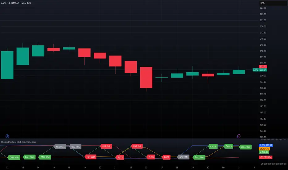
Chaikin Oscillator Multi-Timeframe BiasOverview
Chaikin Oscillator Multi-Timeframe Bias is an indicator designed to help traders align with institutional buying and selling activity by analyzing Chaikin Oscillator signals across two timeframes—a higher timeframe (HTF) for trend bias and a lower timeframe (LTF) for timing. This dual-confirmation model helps traders avoid false breakouts and trade in sync with market momentum and accumulation or distribution dynamics.
Core Concepts
The Chaikin Oscillator measures the momentum of accumulation and distribution based on price and volume. Institutional traders typically accumulate slowly and steadily, and the Chaikin Oscillator helps reveal this pattern. Multi-timeframe analysis confirms whether short-term price action supports the longer-term trend. This indicator applies a smoothing EMA to each Chaikin Oscillator to help confirm direction and reduce noise.
How to Use the Indicator
Start by selecting your timeframes. The higher timeframe, set by default to Daily, establishes the broader directional bias. The lower timeframe, defaulted to 30 minutes, identifies short-term momentum confirmation. The indicator displays one of five labels: CALL Bias, CALL Wait, PUT Bias, PUT Wait, or NEUTRAL. CALL Bias means both HTF and LTF are bullish, signaling a potential opportunity for long or call trades. CALL Wait indicates that the HTF is bullish, but the LTF hasn’t confirmed yet. PUT Bias signals bearish alignment in both HTF and LTF, while PUT Wait indicates HTF is bearish and LTF has not yet confirmed. NEUTRAL means there is no alignment between timeframes and directional trades are not advised.
Interpretation
When the Chaikin Oscillator is above zero and also above its EMA, this indicates bullish momentum and accumulation. When the oscillator is below zero and below its EMA, it suggests bearish momentum and distribution. Bias labels identify when both timeframes are aligned for a higher-probability directional setup. When a “Wait” label appears, it means one timeframe has confirmed bias but the other has not, suggesting the trader should monitor closely but delay entry.
Notes
This indicator includes alerts for both CALL and PUT bias confirmation when both timeframes are aligned. It works on all asset classes, including stocks, ETFs, cryptocurrencies, and futures. Timeframes are fully customizable, and users may explore combinations such as 1D and 1H, or 4H and 15M depending on their strategy. For best results, consider pairing this tool with volume, volatility, or price action analysis.
QG-Particle OscillatorThis is an advanced oscillator based on auxiliary particle filter. It separates signal from noise and uses smoothing algorithm similar to JMA.
The main oscillator line is a smoothed and detrended version of the price series similar to detrended oscillator line. The purple/aqua lines are a prediction based on an additional adaptive smoothing technique and current volatility.
The prediction is smoothed twice and is supposed to represent the true signal without any noise, thus the prediction should always be less than the raw detrend line. However, certain volatile conditions will cause the prediction to cross above/below the detrend line. When this happens the likelihood of a reversal or pullback is extremely high.
There are 3 dots on the zero line- Red, Green and Yellow. The yellow dots warn of an eminent pullback 2 bars before it actually occurs. This is a non-repainting indicator.
One can also use this indicator to trade CCI signals, similar to zero line rejection in existing trend.
The indicator has 2 settings- Period and Phase. The phase represents cycle phase and Period represents oscillator period.
Credits: This indicator has been originally published for Ninjatrader and this is conversion into pinescript.

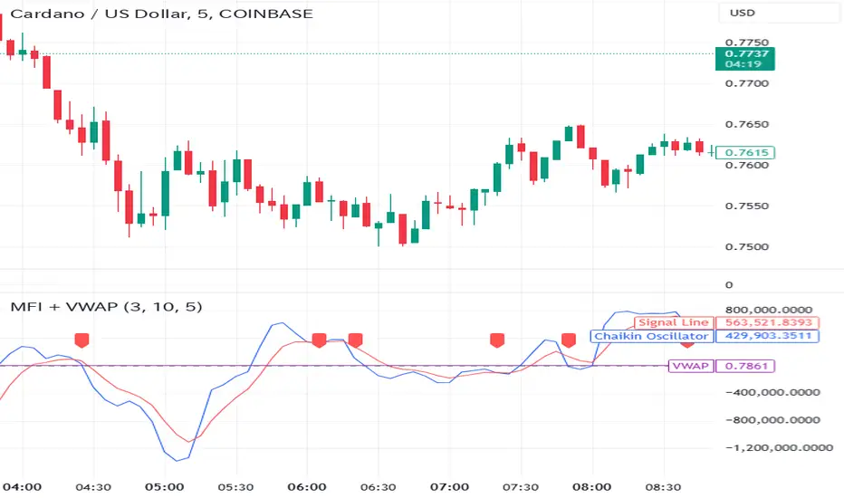
Money Flow Indicator (Chaikin Oscillator) with VWAPStrategy Overview
Entry Conditions:
Buy Entry:
The Chaikin Oscillator crosses above the signal line.
The current price is above the VWAP.
Sell Entry:
The Chaikin Oscillator crosses below the signal line.
The current price is below the VWAP.
Exit Conditions:
Profit Taking:
Take profit when a target profit is reached (e.g., a 2% increase from the entry price).
Stop Loss:
Set a stop loss, for example, at a 1% decline from the entry price.
Risk Management:
Manage risk by limiting each trade to no more than 1-2% of the account balance.
Calculate position size based on risk and trade accordingly.
Trend Confirmation:
Use other indicators (like moving averages) to confirm the overall trend and focus trades in the direction of the trend.
In an uptrend, prioritize buy entries; in a downtrend, prioritize sell entries.
Specific Trade Scenarios
Example 1: Buy Entry:
Enter a buy position when the Chaikin Oscillator crosses above the signal line and the price is above the VWAP.
Set a stop loss 1% below the entry price and a profit target 2% above the entry price.
Example 2: Sell Entry:
Enter a sell position when the Chaikin Oscillator crosses below the signal line and the price is below the VWAP.
Set a stop loss 1% above the entry price and a profit target 2% below the entry price.
Additional Considerations
Backtesting: Test this strategy with historical data to evaluate performance and make adjustments as needed.
Market Conditions: Pay attention to market volatility and economic indicators, adjusting the trading strategy flexibly.
Psychological Factors: Avoid emotional decisions and follow clear rules when trading.
Bitcoin Log Growth Curve OscillatorThis script presents the oscillator version of the Bitcoin Logarithmic Growth Curve 2024 indicator, offering a new perspective on Bitcoin’s long-term price trajectory.
By transforming the original logarithmic growth curve into an oscillator, this version provides a normalized view of price movements within a fixed range, making it easier to identify overbought and oversold conditions.
For a comprehensive explanation of the mathematical derivation, underlying concepts, and overall development of the Bitcoin Logarithmic Growth Curve, we encourage you to explore our primary script, Bitcoin Logarithmic Growth Curve 2024, available here . This foundational script details the regression-based approach used to model Bitcoin’s long-term price evolution.
Normalization Process
The core principle behind this oscillator lies in the normalization of Bitcoin’s price relative to the upper and lower regression boundaries. By applying Min-Max Normalization, we effectively scale the price into a bounded range, facilitating clearer trend analysis. The normalization follows the formula:
normalized price = (upper regresionline − lower regressionline) / (price − lower regressionline)
This transformation ensures that price movements are always mapped within a fixed range, preventing distortions caused by Bitcoin’s exponential long-term growth. Furthermore, this normalization technique has been applied to each of the confidence interval lines, allowing for a structured and systematic approach to analyzing Bitcoin’s historical and projected price behavior.
By representing the logarithmic growth curve in oscillator form, this indicator helps traders and analysts more effectively gauge Bitcoin’s position within its long-term growth trajectory while identifying potential opportunities based on historical price tendencies.

Regime Classifier Oscillator (AiBitcoinTrend)The Regime Classifier Oscillator (AiBitcoinTrend) is an advanced tool for understanding market structure and detecting dynamic price regimes. By combining filtered price trends, clustering algorithms, and an adaptive oscillator, it provides traders with detailed insights into market phases, including accumulation, distribution, advancement, and decline.
This innovative tool simplifies market regime classification, enabling traders to align their strategies with evolving market conditions effectively.
👽 What is a Regime Classifier, and Why is it Useful?
A Regime Classifier is a concept in financial analysis that identifies distinct market conditions or "regimes" based on price behavior and volatility. These regimes often correspond to specific phases of the market, such as trends, consolidations, or periods of high or low volatility. By classifying these regimes, traders and analysts can better understand the underlying market dynamics, allowing them to adapt their strategies to suit prevailing conditions.
👽 Common Uses in Finance
Risk Management: Identifying high-volatility regimes helps traders adjust position sizes or hedge risks.
Strategy Optimization: Traders tailor their approaches—trend-following strategies in trending regimes, mean-reversion strategies in consolidations.
Forecasting: Understanding the current regime aids in predicting potential transitions, such as a shift from accumulation to an upward breakout.
Portfolio Allocation: Investors allocate assets differently based on market regimes, such as increasing cash positions in high-volatility environments.
👽 Why It’s Important
Markets behave differently under varying conditions. A regime classifier provides a structured way to analyze these changes, offering a systematic approach to decision-making. This improves both accuracy and confidence in navigating diverse market scenarios.
👽 How We Implemented the Regime Classifier in This Indicator
The Regime Classifier Oscillator takes the foundational concept of market regime classification and enhances it with advanced computational techniques, making it highly adaptive.
👾 Median Filtering: We smooth price data using a custom median filter to identify significant trends while eliminating noise. This establishes a baseline for price movement analysis.
👾 Clustering Model: Using clustering techniques, the indicator classifies volatility and price trends into distinct regimes:
Advance: Strong upward trends with low volatility.
Decline: Downward trends marked by high volatility.
Accumulation: Consolidation phases with subdued volatility.
Distribution: Topping or bottoming patterns with elevated volatility.
This classification leverages historical price data to refine cluster boundaries dynamically, ensuring adaptive and accurate detection of market states.
Volatility Classification: Price volatility is analyzed through rolling windows, separating data into high and low volatility clusters using distance-based assignments.
Price Trends: The interaction of price levels with the filtered trendline and volatility clusters determines whether the market is advancing, declining, accumulating, or distributing.
👽 Dynamic Cycle Oscillator (DCO):
Captures cyclic behavior and overlays it with smoothed oscillations, providing real-time feedback on price momentum and potential reversals.
Regime Visualization:
Regimes are displayed with intuitive labels and background colors, offering clear, actionable insights directly on the chart.
👽 Why This Implementation Stands Out
Dynamic and Adaptive: The clustering and refit mechanisms adapt to changing market conditions, ensuring relevance across different asset classes and timeframes.
Comprehensive Insights: By combining price trends, volatility, and cyclic behaviors, the indicator provides a holistic view of the market.
This implementation bridges the gap between theoretical regime classification and practical trading needs, making it a powerful tool for both novice and experienced traders.
👽 Applications
👾 Regime-Based Trading Strategies
Traders can use the regime classifications to adapt their strategies effectively:
Advance & Accumulation: Favorable for entering or holding long positions.
Decline & Distribution: Opportunities for short positions or risk management.
👾 Oscillator Insights for Trend Analysis
Overbought/oversold conditions: Early warning of potential reversals.
Dynamic trends: Highlights the strength of price momentum.
👽 Indicator Settings
👾 Filter and Classification Settings
Filter Window Size: Controls trend detection sensitivity.
ATR Lookback: Adjusts the threshold for regime classification.
Clustering Window & Refit Interval: Fine-tunes regime accuracy.
👾 Oscillator Settings
Dynamic Cycle Oscillator Lookback: Defines the sensitivity of cycle detection.
Smoothing Factor: Balances responsiveness and stability.
Disclaimer: This information is for entertainment purposes only and does not constitute financial advice. Please consult with a qualified financial advisor before making any investment decisions.

DR Oscillator 8 * Measures price deviation: Calculates the percentage difference between the closing price and a simple moving average.
* Defines upper and lower limits: User-defined upper and lower limits determine overbought and oversold conditions.
* Signal line: A simple moving average of the deviation is plotted as a signal line.
* Deviation smoothing (optional): The deviation can be smoothed using a moving average to create a smoother line.
* Additional signal line (optional): An additional signal line can be added for further analysis.
* Visual representation: The oscillator is plotted with different colors to indicate overbought, oversold, or neutral conditions.
* Background coloring: The background color changes based on the oscillator's value to provide visual cues for buy or sell signals.
In summary:
The DR Oscillator helps traders identify potential buying and selling opportunities by measuring the extent to which a security's price has deviated from its moving average. When the oscillator moves above the upper limit, it suggests that the asset may be overbought and due for a price correction. Conversely, when it moves below the lower limit, it may indicate an oversold condition and a potential buying opportunity.
However, it's important to note that the DR Oscillator is just one tool and should be used in conjunction with other technical indicators and fundamental analysis for more accurate trading decisions.
