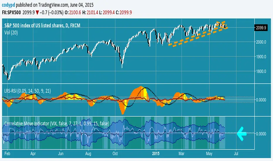
Correlative Move IndicatorEDIT: When loading this indicator it uses a default symbol for comparison of SPX. On Tradingview SPX is a Daily price (unless you buy real time) so you will see "Loading ..." and never see data. Move out to a daily time frame -or- switch the symbol to something available intraday. /EDIT
Correlates the movement of the price you are graphing to the price of someting else that you pick (default is SPX, see EDIT above)
Comments in code explain what I did. If correlations are too tight for CC to show anything but a flat line try this.
Please comment / improve.
=====================
// A simple indicator that looks complex (impress your friends)
// Provides rate of change in the propensity of something
// to move in correlation with whatever you are graphing.
// Inputs are:
// "Compared symbol" - standard Trading View symbol input. You can input ratios & formulas if you like; Defaults to SPX
// "Invert?" - by default the indicator shows the item you have charted as numerator and the "Compared symbol"
// the denominator. So if you graphed "UVXY" and open this indicator with default compared symbol "SPX" then
// the base relationship is UVXY/SPX. Click the box if you want SPX/UVXY (for example) instead.
// "Fast EMA Period" - the period for the fast EMA (white line). default = 7
// "Slow EMA Period" - the period for the slow EMA (black line). default = 27. Important: the bakground color of the indicator
// changes based on this EMA hitting threshold values below.
// "+ threshold" - > threshold for green background. default = 1.0
// "- threshold" - < threshold for red background. default = 0.99
// "BBand Period" - number of periods back for BBand (1 std deviation) calculation. default = 15
// Does not measure correlation per se - it measures change in that correlation.
// If two things do not correlate well in the first place then you will see a lot of noise
// and I wish you much luck in interpreting it.
// However, if two things do correlate well (like VXX and VIX) then this will help you detect
// circumstances where that correlation is unstable. Such instability can signal change in direction.
// I developed it to track real time changes in contango / backwardation in various VIX futures instruments which I trade.
// Tip - always try invert - sometimes the correlation changes become clearer. That can be because the threshold bias
// towards "+" with the defaults here, so think about what the "logical" relationship is and adjust the thresholds, or invert,
// or do both. Just remember - the indicator is below the item you are charting, so the default "source"/"compared"
// relationship is intuitive as you look at the screen. Volatility traders, however, will find "invert" useful with default
// thresholds signalling "green" for contango and "red" for backwardation.
// Short and long ema trends added for smoothing and trend change indications.
// Background color changes to green when correlation changing "positively" and red when "negatively" and white when near 1.
// Think of the value "1" as representing the base "1 to 1" correlation between two things. That doesn't mean same price -
// it means same rate and direction in change in price.
// 1 std deviation is used to build a basic Bollinger Band in blue. The number of periods for calculating that is an input.
// You may find a change in correlation signal outside a Bollinger Band signals a direction change. TV alerts can be
// set for such events.
Tìm kiếm tập lệnh với "vix"
CM ATR PercentileRankCM ATR PercentileRank - Great For Showing Market Bottoms.
When Increased Volatility to the Downside Reaches Extreme Levels it’s Usually a Sign of a Market Bottom.
This Indicator Takes the ATR and uses a different LookBack Period to calculate the Percentile Rank of ATR Which is a Great Way To Calculate Volatility
Be Careful Of Using w/ Market Tops. Not As Reliable.
***Ability to Control ATR Period and set PercentileRank to Different Lookback Period
***Ability to Plot Histogram Just Showing Percentiles or Histogram Based on Up/Down Close
Fuchsia Lines = Greater Than 90th Percentile of Volatility based on ATR and LookBack Period.
Red Lines = Warning — 80-90th Percentile
Orange Lines = 70-80th Percentile
Other Useful Indicators
Williams Vix Fix
CM_RSI EMA Is a Great Filter for Williams Vix Fix

Flat Day PredictorAdvanced technical indicator that predicts low-volatility "flat" trading days using multi-factor analysis. Designed for day traders and scalpers who need to identify when markets are likely to trade sideways.
Key Features:
Real-time flat day probability calculation (0-100%)
8-factor scoring system combining volatility, volume, and momentum indicators
Visual table displaying all indicator values and overall signal strength
Color-coded alerts for high-probability flat day signals
Works on all timeframes, optimized for intraday trading
Indicators Analyzed:
VIX volatility levels
Bollinger Band width compression
RSI momentum neutrality
ATR trend declining
Volume below average
Daily range percentage
Price action patterns
Market regime detection
Signal Levels:
75%+ = VERY HIGH flat probability (Red alert)
62-74% = HIGH flat probability (Orange)
50-61% = MODERATE flat probability (Yellow)
Below 50% = Trending day likely (Green)
Usage:
Add to any chart and monitor the probability percentage. Higher scores indicate increased likelihood of sideways price action. Use for position sizing, strategy selection, and risk management during low-volatility periods.

Opening Range IndicatorComplete Trading Guide: Opening Range Breakout Strategy
What Are Opening Ranges?
Opening ranges capture the high and low prices during the first few minutes of market open. These levels often act as key support and resistance throughout the trading day because:
Heavy volume occurs at market open as overnight orders execute
Institutional activity is concentrated during opening minutes
Price discovery happens as market participants react to overnight news
Psychological levels are established that traders watch all day
Understanding the Three Timeframes
OR5 (5-Minute Range: 9:30-9:35 AM)
Most sensitive - captures immediate market reaction
Quick signals but higher false breakout rate
Best for scalping and momentum trading
Use for early entry when conviction is high
OR15 (15-Minute Range: 9:30-9:45 AM)
Balanced approach - most popular among day traders
Moderate sensitivity with better reliability
Good for swing trades lasting several hours
Primary timeframe for most strategies
OR30 (30-Minute Range: 9:30-10:00 AM)
Most reliable but slower signals
Lower false breakout rate
Best for position trades and trend following
Use when looking for major moves
Core Trading Strategies
Strategy 1: Basic Breakout
Setup:
Wait for price to break above OR15 high or below OR15 low
Enter on the breakout candle close
Stop loss: Opposite side of the range
Target: 2-3x the range size
Example:
OR15 range: $100.00 - $102.00 (Range = $2.00)
Long entry: Break above $102.00
Stop loss: $99.50 (below OR15 low)
Target: $104.00+ (2x range size)
Strategy 2: Multiple Confirmation
Setup:
Wait for OR5 break first (early signal)
Confirm with OR15 break in same direction
Enter on OR15 confirmation
Stop: Below OR30 if available, or OR15 opposite level
Why it works:
Multiple timeframe confirmation reduces false signals and increases probability of sustained moves.
Strategy 3: Failed Breakout Reversal
Setup:
Price breaks OR15 level but fails to hold
Wait for re-entry into the range
Enter reversal trade toward opposite OR level
Stop: Recent breakout high/low
Target: Opposite side of range + extension
Key insight: Failed breakouts often lead to strong moves in the opposite direction.
Advanced Techniques
Range Quality Assessment
High-Quality Ranges (Trade these):
Range size: 0.5% - 2% of stock price
Clean boundaries (not choppy)
Volume spike during range formation
Clear rejection at range levels
Low-Quality Ranges (Avoid these):
Very narrow ranges (<0.3% of stock price)
Extremely wide ranges (>3% of stock price)
Choppy, overlapping candles
Low volume during formation
Volume Confirmation
For Breakouts:
Look for volume spike (2x+ average) on breakout
Declining volume often signals false breakout
Rising volume during range formation shows interest
Market Context Filters
Best Conditions:
Trending market days (SPY/QQQ with clear direction)
Earnings reactions or news-driven moves
High-volume stocks with good liquidity
Volatility above average (VIX considerations)
Avoid Trading When:
Extremely low volume days
Major economic announcements pending
Holidays or half-days
Choppy, sideways market conditions
Risk Management Rules
Position Sizing
Conservative: Risk 0.5% of account per trade
Moderate: Risk 1% of account per trade
Aggressive: Risk 2% maximum per trade
Stop Loss Placement
Inside the range: Quick exit but higher stop-out rate
Outside opposite level: More room but larger risk
ATR-based: 1.5-2x Average True Range below entry
Profit Taking
Target 1: 1x range size (take 50% off)
Target 2: 2x range size (take 25% off)
Runner: Trail remaining 25% with moving stops
Specific Entry Techniques
Breakout Entry Methods
Method 1: Immediate Entry
Enter as soon as price closes above/below range
Fastest entry but highest false signal rate
Best for strong momentum situations
Method 2: Pullback Entry
Wait for breakout, then pullback to range level
Enter when price bounces off former resistance/support
Better risk/reward but may miss some moves
Method 3: Volume Confirmation
Wait for breakout + volume spike
Enter after volume confirmation candle
Reduces false signals significantly
Multiple Timeframe Entries
Aggressive: OR5 break → immediate entry
Conservative: OR5 + OR15 + OR30 all align → enter
Balanced: OR15 break with OR30 support → enter
Common Mistakes to Avoid
1. Trading Poor-Quality Ranges
❌ Don't trade ranges that are too narrow or too wide
✅ Focus on clean, well-defined ranges with good volume
2. Ignoring Volume
❌ Don't chase breakouts without volume confirmation
✅ Always check for volume spike on breakouts
3. Over-Trading
❌ Don't force trades when ranges are unclear
✅ Wait for high-probability setups only
4. Poor Risk Management
❌ Don't risk more than planned or use tight stops in volatile conditions
✅ Stick to predetermined risk levels
5. Fighting the Trend
❌ Don't fade breakouts in strongly trending markets
✅ Align trades with overall market direction
Daily Trading Routine
Pre-Market (8:00-9:30 AM)
Check overnight news and earnings
Review major indices (SPY, QQQ, IWM)
Identify potential opening range candidates
Set alerts for range breakouts
Market Open (9:30-10:00 AM)
Watch opening range formation
Note volume and price action quality
Mark key levels on charts
Prepare for breakout signals
Trading Session (10:00 AM - 4:00 PM)
Execute breakout strategies
Manage existing positions
Trail stops as profits develop
Look for additional setups
Post-Market Review
Analyze winning and losing trades
Review range quality vs. outcomes
Identify improvement areas
Prepare for next session
Best Stocks/ETFs for Opening Range Trading
Large Cap Stocks (Best for beginners):
AAPL, MSFT, GOOGL, AMZN, TSLA
High liquidity, predictable behavior
Good range formation most days
ETFs (Consistent patterns):
SPY, QQQ, IWM, XLF, XLE
Excellent liquidity
Clear range boundaries
Mid-Cap Growth (Advanced traders):
Stocks with good volume (1M+ shares daily)
Recent news catalysts
Clean technical patterns
Performance Optimization
Track These Metrics:
Win rate by range type (OR5 vs OR15 vs OR30)
Average R/R (risk vs reward ratio)
Best performing market conditions
Time of day performance
Continuous Improvement:
Keep detailed trade journal
Review failed breakouts for patterns
Adjust position sizing based on win rate
Refine entry timing based on backtesting
Final Tips for Success
Start small - Paper trade or use tiny positions initially
Focus on quality - Better to miss trades than take bad ones
Stay disciplined - Stick to your rules even during losing streaks
Adapt to conditions - What works in trending markets may fail in choppy conditions
Keep learning - Markets evolve, so should your approach
The opening range strategy is powerful because it captures natural market behavior, but like all strategies, it requires practice, discipline, and proper risk management to be profitable long-term.

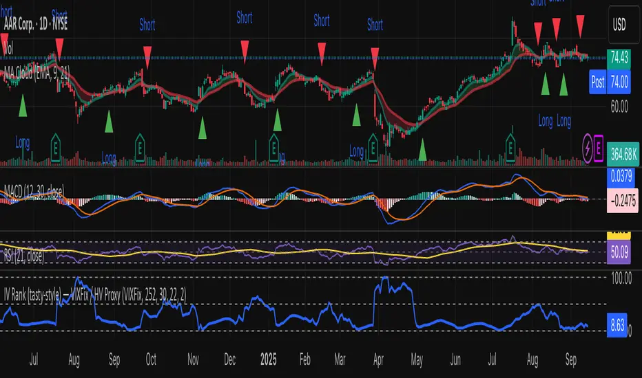
IV Rank (tasty-style) — VIXFix / HV ProxyIV Rank (tasty-style) — VIXFix / HV Proxy
Overview
This indicator replicates tastytrade’s IV Rank calculation—but built entirely inside TradingView.
Because TradingView does not expose live option-chain implied volatility, the script lets you choose between two widely used price-based IV proxies:
VIXFix (Williams VIX Fix): a fast-reacting volatility estimate derived from price extremes.
HV(30): 30-day annualized historical volatility of daily log returns.
The goal is to approximate the “rich vs. cheap” option volatility environment that traders use to decide whether to sell or buy premium.
Formula
IV Rank answers the question: Where is current implied volatility relative to its own 1-year range?
𝐼
𝑉
𝑅
=
𝐼
𝑉
𝑐
𝑢
𝑟
𝑟
𝑒
𝑛
𝑡
−
𝐼
𝑉
1
𝑦
𝐿
𝑜
𝑤
𝐼
𝑉
1
𝑦
𝐻
𝑖
𝑔
ℎ
−
𝐼
𝑉
1
𝑦
𝐿
𝑜
𝑤
×
100
IVR=
IV
1yHigh
−IV
1yLow
IV
current
−IV
1yLow
×100
IVcurrent: Current value of the chosen IV proxy.
IV1yHigh/Low: Highest and lowest proxy values over the user-defined lookback (default 252 trading days ≈ 1 year).
IVR = 0 → Current IV equals its 1-year low
IVR = 100 → Current IV equals its 1-year high
IVR ≈ 50 → Current IV sits mid-range
How to Use
High IV Rank (≥50–60%)
Options are relatively expensive → short-premium strategies (credit spreads, iron condors, straddles) may be more attractive.
Low IV Rank (≤20%)
Options are relatively cheap → long-premium strategies (debit spreads, calendars, diagonals) may offer better risk/reward.
Combine with your own analysis, liquidity checks, and risk management.
Inputs & Customization
IV Source: Choose “VIXFix” or “HV(30)” as the volatility proxy.
IVR Lookback: Rolling window for 1-year high/low (default 252 trading days).
VIXFix Parameters: Length and stdev multiplier to fine-tune sensitivity.
Info Label: Optional on-chart label displays current IV proxy, 1-year high/low, and IV Rank.
Alerts: Optional alerts when IVR crosses 50, falls below 20, or rises above 80.
Notes & Limitations
This indicator does not pull real option-chain IV.
It provides a close structural analogue to tastytrade’s IV Rank using price-derived proxies for markets where options data is not directly available.
For live option IV, use broker platforms or third-party data feeds alongside this script.
Tags: IV Rank, Implied Volatility, Tastytrade, VIXFix, Historical Volatility, Options, Premium Selling, Debit Spreads, Market Volatility
B3 – VIX + Breadth + SR + Projeção 14dA comprehensive technical analysis tool that combines volatility proxies (HV, ATR, BB Width, composite VolIndex), market breadth (internal and multi-timeframe), pivot-based support/resistance with strength and confluence, and a 14-day linear regression projection with confidence bands. Designed to provide a holistic view of trend, risk, and key price levels for swing and medium-term trading decisions.

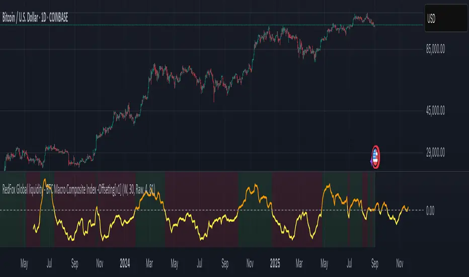
BTC Macro Composite Global liquidity Index -OffsetThis indicator is based on the thesis that Bitcoin price movements are heavily influenced by macro liquidity trends. It calculates a weighted composite index based on the following components:
• Global Liquidity (41%): Sum of central bank balance sheets (Fed , ECB , BoJ , and PBoC ), adjusted to USD.
• Investor Risk Appetite (22%): Derived from the Copper/Gold ratio, inverse VIX (as a risk-on signal), and the spread between High Yield and Investment Grade bonds (HY vs IG OAS).
• Gold Sensitivity (15–20%): Combines the XAUUSD price with BTC/Gold ratio to reflect the historical influence of gold on Bitcoin pricing.
Each component is normalized and then offset forward by 90 days to attempt predictive alignment with Bitcoin’s price.
The goal is to identify macro inflection points with high predictive value for BTC. It is not a trading signal generator but rather a macro trend context indicator.
❗ Important: This script should be used with caution. It does not account for geopolitical shocks, regulatory events, or internal BTC market structure (e.g., miner behavior, on-chain metrics).
💡 How to use:
• Use on the 1D timeframe.
• Look for divergences between BTC price and the macro index.
• Apply in confluence with other technical or fundamental frameworks.
🔍 Originality:
While similar components exist in macro dashboards, this script combines them uniquely using time-forward offsets and custom weighting specifically tailored for BTC behavior.
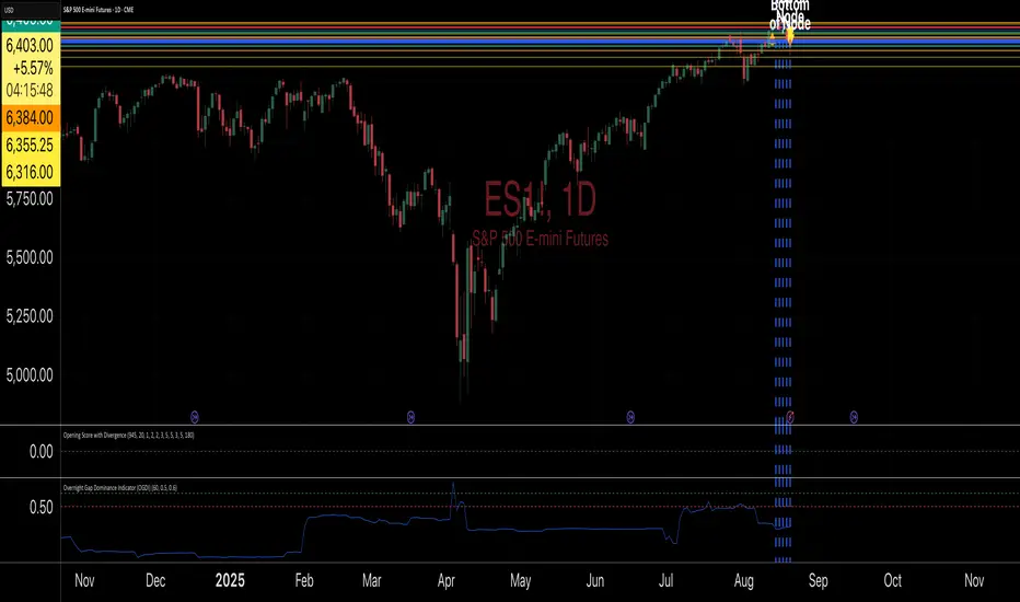
Overnight Gap Dominance Indicator (OGDI)The Overnight Gap Dominance Indicator (OGDI) measures the relative volatility of overnight price gaps versus intraday price movements for a given security, such as SPY or SPX. It uses a rolling standard deviation of absolute overnight percentage changes divided by the standard deviation of absolute intraday percentage changes over a customizable window. This helps traders identify periods where overnight gaps predominate, suggesting potential opportunities for strategies leveraging extended market moves.
Instructions
A
pply the indicator to your TradingView chart for the desired security (e.g., SPY or SPX).
Adjust the "Rolling Window" input to set the lookback period (default: 60 bars).
Modify the "1DTE Threshold" and "2DTE+ Threshold" inputs to tailor the levels at which you switch from 0DTE to 1DTE or multi-DTE strategies (default: 0.5 and 0.6).
Observe the OGDI line: values above the 1DTE threshold suggest favoring 1DTE strategies, while values above the 2DTE+ threshold indicate multi-DTE strategies may be more effective.
Use in conjunction with low VIX environments and uptrend legs for optimal results.
Information-Geometric Market DynamicsInformation-Geometric Market Dynamics
The Information Field: A Geometric Approach to Market Dynamics
By: DskyzInvestments
Foreword: Beyond the Shadows on the Wall
If you have traded for any length of time, you know " the feeling ." It is the frustration of a perfect setup that fails, the whipsaw that stops you out just before the real move, the nagging sense that the chart is telling you only half the story. For decades, technical analysis has relied on interpreting the shadows—the patterns left behind by price. We draw lines on these shadows, apply indicators to them, and hope they reveal the future.
But what if we could stop looking at the shadows and, instead, analyze the object casting them?
This script introduces a new paradigm for market analysis: Information-Geometric Market Dynamics (IGMD) . The core premise of IGMD is that the price chart is merely a one-dimensional projection of a much richer, higher-dimensional reality—an " information field " generated by the collective actions and beliefs of all market participants.
This is not just another collection of indicators. It is a unified framework for measuring the geometry of the market's information field—its memory, its complexity, its uncertainty, its causal flows—and making high-probability decisions based on that deeper reality. By fusing advanced mathematical and informational concepts, IGMD provides a multi-faceted lens through which to view market behavior, moving beyond simple price action into the very structure of market information itself.
Prepare to move beyond the flatland of the price chart. Welcome to the information field.
The IGMD Framework: A Multi-Kernel Approach
What is a Kernel? The Heart of Transformation
In mathematics and data science, a kernel is a powerful and elegant concept. At its core, a kernel is a function that takes complex, often inscrutable data and transforms it into a more useful format. Think of it as a specialized lens or a mathematical "probe." You cannot directly measure abstract concepts like "market memory" or "trend quality" by looking at a price number. First, you must process the raw price data through a specific mathematical machine—a kernel—that is designed to output a measurement of that specific property. Kernels operate by performing a sort of "similarity test," projecting data into a higher-dimensional space where hidden patterns and relationships become visible and measurable.
Why do creators use them? We use kernels to extract features —meaningful pieces of information—that are not explicitly present in the raw data. They are the essential tools for moving beyond surface-level analysis into the very DNA of market behavior. A simple moving average can tell you the average price; a suite of well-chosen kernels can tell you about the character of the price action itself.
The Alchemist's Challenge: The Art of Fusion
Using a single kernel is a challenge. Using five distinct, computationally demanding mathematical engines in unison is an immense undertaking. The true difficulty—and artistry—lies not just in using one kernel, but in fusing the outputs of many . Each kernel provides a different perspective, and they can often give conflicting signals. One kernel might detect a strong trend, while another signals rising chaos and uncertainty. The IGMD script's greatest strength is its ability to act as this alchemist, synthesizing these disparate viewpoints through a weighted fusion process to produce a single, coherent picture of the market's state. It required countless hours of testing and calibration to balance the influence of these five distinct analytical engines so they work in harmony rather than cacophony.
The Five Kernels of Market Dynamics
The IGMD script is built upon a foundation of five distinct kernels, each chosen to probe a unique and critical dimension of the market's information field.
1. The Wavelet Kernel (The "Microscope")
What it is: The Wavelet Kernel is a signal processing function designed to decompose a signal into different frequency scales. Unlike a Fourier Transform that analyzes the entire signal at once, the wavelet slides across the data, providing information about both what frequencies are present and when they occurred.
The Kernels I Use:
Haar Kernel: The simplest wavelet, a square-wave shape defined by the coefficients . It excels at detecting sharp, sudden changes.
Daubechies 2 (db2) Kernel: A more complex and smoother wavelet shape that provides a better balance for analyzing the nuanced ebb and flow of typical market trends.
How it Works in the Script: This kernel is applied iteratively. It first separates the finest "noise" (detail d1) from the first level of trend (approximation a1). It then takes the trend a1 and repeats the process, extracting the next level of cycle (d2) and trend (a2), and so on. This hierarchical decomposition allows us to separate short-term noise from the long-term market "thesis."
2. The Hurst Exponent Kernel (The "Memory Gauge")
What it is: The Hurst Exponent is derived from a statistical analysis kernel that measures the "long-term memory" or persistence of a time series. It is the definitive measure of whether a series is trending (H > 0.5), mean-reverting (H < 0.5), or random (H = 0.5).
How it Works in the Script: The script employs a method based on Rescaled Range (R/S) analysis. It calculates the average range of price movements over increasingly larger time lags (m1, m2, m4, m8...). The slope of the line plotting log(range) vs. log(lag) is the Hurst Exponent. Applying this complex statistical analysis not to the raw price, but to the clean, wavelet-decomposed trend lines, is a key innovation of IGMD.
3. The Fractal Dimension Kernel (The "Complexity Compass")
What it is: This kernel measures the geometric complexity or "jaggedness" of a price path, based on the principles of fractal geometry. A straight line has a dimension of 1; a chaotic, space-filling line approaches a dimension of 2.
How it Works in the Script: We use a version based on Ehlers' Fractal Dimension Index (FDI). It calculates the rate of price change over a full lookback period (N3) and compares it to the sum of the rates of change over the two halves of that period (N1 + N2). The formula d = (log(N1 + N2) - log(N3)) / log(2) quantifies how much "longer" and more convoluted the price path was than a simple straight line. This kernel is our primary filter for tradeable (low complexity) vs. untradeable (high complexity) conditions.
4. The Shannon Entropy Kernel (The "Uncertainty Meter")
What it is: This kernel comes from Information Theory and provides the purest mathematical measure of information, surprise, or uncertainty within a system. It is not a measure of volatility; a market moving predictably up by 10 points every bar has high volatility but zero entropy .
How it Works in the Script: The script normalizes price returns by the ATR, categorizes them into a discrete number of "bins" over a lookback window, and forms a probability distribution. The Shannon Entropy H = -Σ(p_i * log(p_i)) is calculated from this distribution. A low H means returns are predictable. A high H means returns are chaotic. This kernel is our ultimate gauge of market conviction.
5. The Transfer Entropy Kernel (The "Causality Probe")
What it is: This is by far the most advanced and computationally intensive kernel in the script. Transfer Entropy is a non-parametric measure of directed information flow between two time series. It moves beyond correlation to ask: "Does knowing the past of Volume genuinely reduce our uncertainty about the future of Price?"
How it Works in the Script: To make this work, the script discretizes both price returns and the chosen "driver" (e.g., OBV) into three states: "up," "down," or "neutral." It then builds complex conditional probability tables to measure the flow of information in both directions. The Net Transfer Entropy (TE Driver→Price minus TE Price→Driver) gives us a direct measure of causality . A positive score means the driver is leading price, confirming the validity of the move. This is a profound leap beyond traditional indicator analysis.
Chapter 3: Fusion & Interpretation - The Field Score & Dashboard
Each kernel is a specialist providing a piece of the puzzle. The Field Score is where they are fused into a single, comprehensive reading. It's a weighted sum of the normalized scores from all five kernels, producing a single number from -1 (maximum bearish information field) to +1 (maximum bullish information field). This is the ultimate "at-a-glance" metric for the market's net state, and it is interpreted through the dashboard.
The Dashboard: Your Mission Control
Field Score & Regime: The master metric and its plain-English interpretation ("Uptrend Field", "Downtrend Field", "Transitional").
Kernel Readouts (Wave Align, H(w), FDI, etc.): The live scores of each individual kernel. This allows you to see why the Field Score is what it is. A high Field Score with all components in agreement (all green or red) is a state of High Coherence and represents a high-quality setup.
Market Context: Standard metrics like RSI and Volume for additional confluence.
Signals: The raw and adjusted confluence counts and the final, calculated probability scores for potential long and short entries.
Pattern: Shows the dominant candlestick pattern detected within the currently forming APEX range box and its calculated confidence percentage.
Chapter 4: Mastering the Controls - The Inputs Menu
Every parameter is a lever to fine-tune the IGMD engine.
📊 Wavelet Transform: Kernel ( Haar for sharp moves, db2 for smooth trends) and Scales (depth of analysis) let you tune the script's core microscope to your asset's personality.
📈 Hurst Exponent: The Window determines if you're assessing short-term or long-term market memory.
🔍 Fractal Dimension & ⚡ Entropy Volatility: Adjust the lookback windows to make these kernels more or less sensitive to recent price action. Always keep "Normalize by ATR" enabled for Entropy for consistent results.
🔄 Transfer Entropy: Driver lets you choose what causal force to measure (e.g., OBV, Volume, or even an external symbol like VIX). The throttle setting is a crucial performance tool, allowing you to balance precision with script speed.
⚡ Field Fusion • Weights: This is where you can customize the model's "brain." Increase the weights for the kernels that best align with your trading philosophy (e.g., w_hurst for trend followers, w_fdi for chop avoiders).
📊 Signal Engine: Mode offers presets from Conservative to Aggressive . Min Confluence sets your evidence threshold. Dynamic Confluence is a powerful feature that automatically adapts this threshold to the market regime.
🎨 Visuals & 📏 Support/Resistance: These inputs give you full control over the chart's appearance, allowing you to toggle every visual element for a setup that is as clean or as data-rich as you desire.
Chapter 5: Reading the Battlefield - On-Chart Visuals
Pattern Boxes (The Large Rectangles): These are not simple range boxes. They appear when the Field Score crosses a significance threshold, signaling a potential ignition point.
Color: The color reflects the dominant candlestick pattern that has occurred within that box's duration (e.g., green for Bull Engulf).
Label: Displays the dominant pattern, its duration in bars, and a calculated Confidence % based on field strength and pattern clarity.
Bar Pattern Boxes (The Small Boxes): If enabled, these highlight individual, significant candlestick patterns ( BE for Bull Engulf, H for Hammer) on a bar-by-bar basis.
Signal Markers (▲ and ▼): These appear only when the Signal Engine's criteria are all met. The number is the calculated Probability Score .
RR Rails (Dashed Lines): When a signal appears, these lines automatically plot the Entry, Stop Loss (based on ATR), and two Take Profit targets (based on Risk/Reward ratios). They dynamically break and disappear as price touches each level.
Support & Resistance Lines: Plots of the highest high ( Resistance ) and lowest low ( Support ) over a lookback, providing key structural levels.
Chapter 6: Development Philosophy & A Final Word
One single question: " What is the market really doing? " It represents a triumph of complexity, blending concepts from signal processing, chaos theory, and information theory into a cohesive framework. It is offered for educational and analytical purposes and does not constitute financial advice. Its goal is to elevate your analysis from interpreting flat shadows to measuring the rich, geometric reality of the market's information field.
As the great mathematician Benoit Mandelbrot , father of fractal geometry, noted:
"Clouds are not spheres, mountains are not cones, coastlines are not circles, and bark is not smooth, nor does lightning travel in a straight line."
Neither does the market. IGMD is a tool designed to navigate that beautiful, complex, and fractal reality.
— Dskyz, Trade with insight. Trade with anticipation.

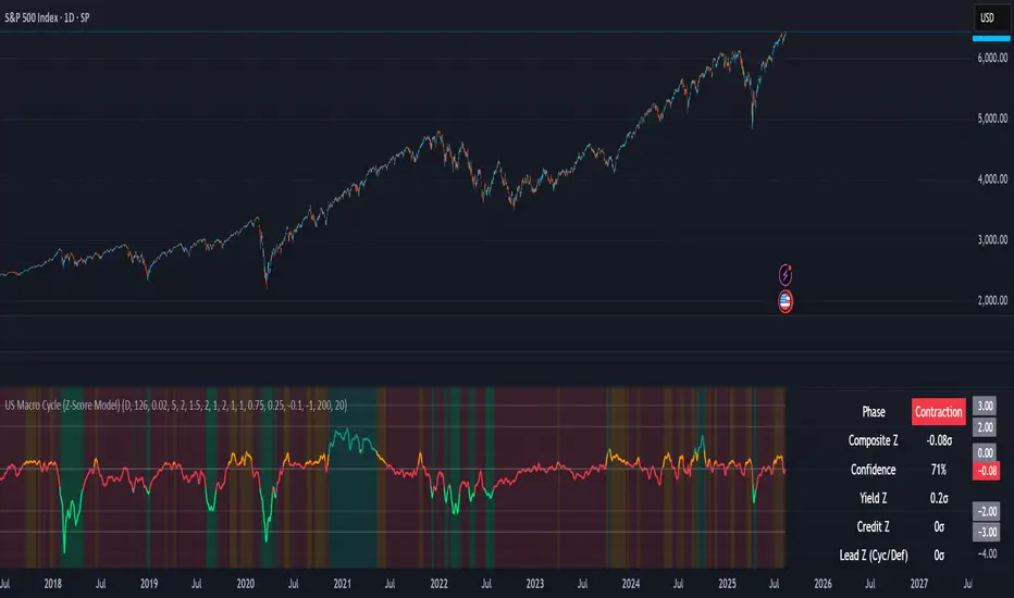
US Macro Cycle (Z-Score Model)US Macro Cycle (Z-Score Model)
This indicator tracks the US economic cycle in real time using a weighted composite of seven macro and market-based indicators, each converted into a rolling Z-score for comparability. The model identifies the current phase of the cycle — Expansion, Peak, Contraction, or Recovery — and suggests sector tilts based on historical performance in each phase.
Core Components:
Yield Curve (10y–2y): Positive & steepening = growth; inverted = slowdown risk.
Credit Spreads (HYG/LQD): Tightening = risk-on; widening = risk-off.
Sector Leadership (Cyclicals vs. Defensives): Measures market leadership regime.
Copper/Gold Ratio: Higher copper = growth signal; higher gold = defensive.
SPY vs. 200-day MA: Equity trend strength.
SPY/IEF Ratio: Stocks vs. bonds relative strength.
VIX (Inverted): Low/falling volatility = supportive; high/rising = risk-off.
Methodology:
Each series is transformed into a rolling Z-score over the selected lookback period (optionally using median/MAD for robustness and winsorization to clip outliers).
Z-scores are combined using user-defined weights and normalized.
The smoothed composite is compared against phase thresholds to classify the macro environment.
Features:
Customizable Weights: Emphasize the indicators most relevant to your strategy.
Adjustable Thresholds: Fine-tune cycle phase definitions.
Background Coloring: Visual cue for the current phase.
Summary Table: Displays composite Z, confidence %, and individual Z-scores.
Alerts: Trigger when the phase changes, with details on the composite score and recommended tilt.
Use Cases:
Align sector rotation or relative strength strategies with the macro backdrop.
Identify favorable or defensive phases for tactical allocation.
Monitor macro turning points to manage portfolio risk.
It's doesn't fill nan gaps so there is quite a bit of zeroes, non-repainting.
Kelly Position Size CalculatorThis position sizing calculator implements the Kelly Criterion, developed by John L. Kelly Jr. at Bell Laboratories in 1956, to determine mathematically optimal position sizes for maximizing long-term wealth growth. Unlike arbitrary position sizing methods, this tool provides a scientifically solution based on your strategy's actual performance statistics and incorporates modern refinements from over six decades of academic research.
The Kelly Criterion addresses a fundamental question in capital allocation: "What fraction of capital should be allocated to each opportunity to maximize growth while avoiding ruin?" This question has profound implications for financial markets, where traders and investors constantly face decisions about optimal capital allocation (Van Tharp, 2007).
Theoretical Foundation
The Kelly Criterion for binary outcomes is expressed as f* = (bp - q) / b, where f* represents the optimal fraction of capital to allocate, b denotes the risk-reward ratio, p indicates the probability of success, and q represents the probability of loss (Kelly, 1956). This formula maximizes the expected logarithm of wealth, ensuring maximum long-term growth rate while avoiding the risk of ruin.
The mathematical elegance of Kelly's approach lies in its derivation from information theory. Kelly's original work was motivated by Claude Shannon's information theory (Shannon, 1948), recognizing that maximizing the logarithm of wealth is equivalent to maximizing the rate of information transmission. This connection between information theory and wealth accumulation provides a deep theoretical foundation for optimal position sizing.
The logarithmic utility function underlying the Kelly Criterion naturally embodies several desirable properties for capital management. It exhibits decreasing marginal utility, penalizes large losses more severely than it rewards equivalent gains, and focuses on geometric rather than arithmetic mean returns, which is appropriate for compounding scenarios (Thorp, 2006).
Scientific Implementation
This calculator extends beyond basic Kelly implementation by incorporating state of the art refinements from academic research:
Parameter Uncertainty Adjustment: Following Michaud (1989), the implementation applies Bayesian shrinkage to account for parameter estimation error inherent in small sample sizes. The adjustment formula f_adjusted = f_kelly × confidence_factor + f_conservative × (1 - confidence_factor) addresses the overconfidence bias documented by Baker and McHale (2012), where the confidence factor increases with sample size and the conservative estimate equals 0.25 (quarter Kelly).
Sample Size Confidence: The reliability of Kelly calculations depends critically on sample size. Research by Browne and Whitt (1996) provides theoretical guidance on minimum sample requirements, suggesting that at least 30 independent observations are necessary for meaningful parameter estimates, with 100 or more trades providing reliable estimates for most trading strategies.
Universal Asset Compatibility: The calculator employs intelligent asset detection using TradingView's built-in symbol information, automatically adapting calculations for different asset classes without manual configuration.
ASSET SPECIFIC IMPLEMENTATION
Equity Markets: For stocks and ETFs, position sizing follows the calculation Shares = floor(Kelly Fraction × Account Size / Share Price). This straightforward approach reflects whole share constraints while accommodating fractional share trading capabilities.
Foreign Exchange Markets: Forex markets require lot-based calculations following Lot Size = Kelly Fraction × Account Size / (100,000 × Base Currency Value). The calculator automatically handles major currency pairs with appropriate pip value calculations, following industry standards described by Archer (2010).
Futures Markets: Futures position sizing accounts for leverage and margin requirements through Contracts = floor(Kelly Fraction × Account Size / Margin Requirement). The calculator estimates margin requirements as a percentage of contract notional value, with specific adjustments for micro-futures contracts that have smaller sizes and reduced margin requirements (Kaufman, 2013).
Index and Commodity Markets: These markets combine characteristics of both equity and futures markets. The calculator automatically detects whether instruments are cash-settled or futures-based, applying appropriate sizing methodologies with correct point value calculations.
Risk Management Integration
The calculator integrates sophisticated risk assessment through two primary modes:
Stop Loss Integration: When fixed stop-loss levels are defined, risk calculation follows Risk per Trade = Position Size × Stop Loss Distance. This ensures that the Kelly fraction accounts for actual risk exposure rather than theoretical maximum loss, with stop-loss distance measured in appropriate units for each asset class.
Strategy Drawdown Assessment: For discretionary exit strategies, risk estimation uses maximum historical drawdown through Risk per Trade = Position Value × (Maximum Drawdown / 100). This approach assumes that individual trade losses will not exceed the strategy's historical maximum drawdown, providing a reasonable estimate for strategies with well-defined risk characteristics.
Fractional Kelly Approaches
Pure Kelly sizing can produce substantial volatility, leading many practitioners to adopt fractional Kelly approaches. MacLean, Sanegre, Zhao, and Ziemba (2004) analyze the trade-offs between growth rate and volatility, demonstrating that half-Kelly typically reduces volatility by approximately 75% while sacrificing only 25% of the growth rate.
The calculator provides three primary Kelly modes to accommodate different risk preferences and experience levels. Full Kelly maximizes growth rate while accepting higher volatility, making it suitable for experienced practitioners with strong risk tolerance and robust capital bases. Half Kelly offers a balanced approach popular among professional traders, providing optimal risk-return balance by reducing volatility significantly while maintaining substantial growth potential. Quarter Kelly implements a conservative approach with low volatility, recommended for risk-averse traders or those new to Kelly methodology who prefer gradual introduction to optimal position sizing principles.
Empirical Validation and Performance
Extensive academic research supports the theoretical advantages of Kelly sizing. Hakansson and Ziemba (1995) provide a comprehensive review of Kelly applications in finance, documenting superior long-term performance across various market conditions and asset classes. Estrada (2008) analyzes Kelly performance in international equity markets, finding that Kelly-based strategies consistently outperform fixed position sizing approaches over extended periods across 19 developed markets over a 30-year period.
Several prominent investment firms have successfully implemented Kelly-based position sizing. Pabrai (2007) documents the application of Kelly principles at Berkshire Hathaway, noting Warren Buffett's concentrated portfolio approach aligns closely with Kelly optimal sizing for high-conviction investments. Quantitative hedge funds, including Renaissance Technologies and AQR, have incorporated Kelly-based risk management into their systematic trading strategies.
Practical Implementation Guidelines
Successful Kelly implementation requires systematic application with attention to several critical factors:
Parameter Estimation: Accurate parameter estimation represents the greatest challenge in practical Kelly implementation. Brown (1976) notes that small errors in probability estimates can lead to significant deviations from optimal performance. The calculator addresses this through Bayesian adjustments and confidence measures.
Sample Size Requirements: Users should begin with conservative fractional Kelly approaches until achieving sufficient historical data. Strategies with fewer than 30 trades may produce unreliable Kelly estimates, regardless of adjustments. Full confidence typically requires 100 or more independent trade observations.
Market Regime Considerations: Parameters that accurately describe historical performance may not reflect future market conditions. Ziemba (2003) recommends regular parameter updates and conservative adjustments when market conditions change significantly.
Professional Features and Customization
The calculator provides comprehensive customization options for professional applications:
Multiple Color Schemes: Eight professional color themes (Gold, EdgeTools, Behavioral, Quant, Ocean, Fire, Matrix, Arctic) with dark and light theme compatibility ensure optimal visibility across different trading environments.
Flexible Display Options: Adjustable table size and position accommodate various chart layouts and user preferences, while maintaining analytical depth and clarity.
Comprehensive Results: The results table presents essential information including asset specifications, strategy statistics, Kelly calculations, sample confidence measures, position values, risk assessments, and final position sizes in appropriate units for each asset class.
Limitations and Considerations
Like any analytical tool, the Kelly Criterion has important limitations that users must understand:
Stationarity Assumption: The Kelly Criterion assumes that historical strategy statistics represent future performance characteristics. Non-stationary market conditions may invalidate this assumption, as noted by Lo and MacKinlay (1999).
Independence Requirement: Each trade should be independent to avoid correlation effects. Many trading strategies exhibit serial correlation in returns, which can affect optimal position sizing and may require adjustments for portfolio applications.
Parameter Sensitivity: Kelly calculations are sensitive to parameter accuracy. Regular calibration and conservative approaches are essential when parameter uncertainty is high.
Transaction Costs: The implementation incorporates user-defined transaction costs but assumes these remain constant across different position sizes and market conditions, following Ziemba (2003).
Advanced Applications and Extensions
Multi-Asset Portfolio Considerations: While this calculator optimizes individual position sizes, portfolio-level applications require additional considerations for correlation effects and aggregate risk management. Simplified portfolio approaches include treating positions independently with correlation adjustments.
Behavioral Factors: Behavioral finance research reveals systematic biases that can interfere with Kelly implementation. Kahneman and Tversky (1979) document loss aversion, overconfidence, and other cognitive biases that lead traders to deviate from optimal strategies. Successful implementation requires disciplined adherence to calculated recommendations.
Time-Varying Parameters: Advanced implementations may incorporate time-varying parameter models that adjust Kelly recommendations based on changing market conditions, though these require sophisticated econometric techniques and substantial computational resources.
Comprehensive Usage Instructions and Practical Examples
Implementation begins with loading the calculator on your desired trading instrument's chart. The system automatically detects asset type across stocks, forex, futures, and cryptocurrency markets while extracting current price information. Navigation to the indicator settings allows input of your specific strategy parameters.
Strategy statistics configuration requires careful attention to several key metrics. The win rate should be calculated from your backtest results using the formula of winning trades divided by total trades multiplied by 100. Average win represents the sum of all profitable trades divided by the number of winning trades, while average loss calculates the sum of all losing trades divided by the number of losing trades, entered as a positive number. The total historical trades parameter requires the complete number of trades in your backtest, with a minimum of 30 trades recommended for basic functionality and 100 or more trades optimal for statistical reliability. Account size should reflect your available trading capital, specifically the risk capital allocated for trading rather than total net worth.
Risk management configuration adapts to your specific trading approach. The stop loss setting should be enabled if you employ fixed stop-loss exits, with the stop loss distance specified in appropriate units depending on the asset class. For stocks, this distance is measured in dollars, for forex in pips, and for futures in ticks. When stop losses are not used, the maximum strategy drawdown percentage from your backtest provides the risk assessment baseline. Kelly mode selection offers three primary approaches: Full Kelly for aggressive growth with higher volatility suitable for experienced practitioners, Half Kelly for balanced risk-return optimization popular among professional traders, and Quarter Kelly for conservative approaches with reduced volatility.
Display customization ensures optimal integration with your trading environment. Eight professional color themes provide optimization for different chart backgrounds and personal preferences. Table position selection allows optimal placement within your chart layout, while table size adjustment ensures readability across different screen resolutions and viewing preferences.
Detailed Practical Examples
Example 1: SPY Swing Trading Strategy
Consider a professionally developed swing trading strategy for SPY (S&P 500 ETF) with backtesting results spanning 166 total trades. The strategy achieved 110 winning trades, representing a 66.3% win rate, with an average winning trade of $2,200 and average losing trade of $862. The maximum drawdown reached 31.4% during the testing period, and the available trading capital amounts to $25,000. This strategy employs discretionary exits without fixed stop losses.
Implementation requires loading the calculator on the SPY daily chart and configuring the parameters accordingly. The win rate input receives 66.3, while average win and loss inputs receive 2200 and 862 respectively. Total historical trades input requires 166, with account size set to 25000. The stop loss function remains disabled due to the discretionary exit approach, with maximum strategy drawdown set to 31.4%. Half Kelly mode provides the optimal balance between growth and risk management for this application.
The calculator generates several key outputs for this scenario. The risk-reward ratio calculates automatically to 2.55, while the Kelly fraction reaches approximately 53% before scientific adjustments. Sample confidence achieves 100% given the 166 trades providing high statistical confidence. The recommended position settles at approximately 27% after Half Kelly and Bayesian adjustment factors. Position value reaches approximately $6,750, translating to 16 shares at a $420 SPY price. Risk per trade amounts to approximately $2,110, representing 31.4% of position value, with expected value per trade reaching approximately $1,466. This recommendation represents the mathematically optimal balance between growth potential and risk management for this specific strategy profile.
Example 2: EURUSD Day Trading with Stop Losses
A high-frequency EURUSD day trading strategy demonstrates different parameter requirements compared to swing trading approaches. This strategy encompasses 89 total trades with a 58% win rate, generating an average winning trade of $180 and average losing trade of $95. The maximum drawdown reached 12% during testing, with available capital of $10,000. The strategy employs fixed stop losses at 25 pips and take profit targets at 45 pips, providing clear risk-reward parameters.
Implementation begins with loading the calculator on the EURUSD 1-hour chart for appropriate timeframe alignment. Parameter configuration includes win rate at 58, average win at 180, and average loss at 95. Total historical trades input receives 89, with account size set to 10000. The stop loss function is enabled with distance set to 25 pips, reflecting the fixed exit strategy. Quarter Kelly mode provides conservative positioning due to the smaller sample size compared to the previous example.
Results demonstrate the impact of smaller sample sizes on Kelly calculations. The risk-reward ratio calculates to 1.89, while the Kelly fraction reaches approximately 32% before adjustments. Sample confidence achieves 89%, providing moderate statistical confidence given the 89 trades. The recommended position settles at approximately 7% after Quarter Kelly application and Bayesian shrinkage adjustment for the smaller sample. Position value amounts to approximately $700, translating to 0.07 standard lots. Risk per trade reaches approximately $175, calculated as 25 pips multiplied by lot size and pip value, with expected value per trade at approximately $49. This conservative position sizing reflects the smaller sample size, with position sizes expected to increase as trade count surpasses 100 and statistical confidence improves.
Example 3: ES1! Futures Systematic Strategy
Systematic futures trading presents unique considerations for Kelly criterion application, as demonstrated by an E-mini S&P 500 futures strategy encompassing 234 total trades. This systematic approach achieved a 45% win rate with an average winning trade of $1,850 and average losing trade of $720. The maximum drawdown reached 18% during the testing period, with available capital of $50,000. The strategy employs 15-tick stop losses with contract specifications of $50 per tick, providing precise risk control mechanisms.
Implementation involves loading the calculator on the ES1! 15-minute chart to align with the systematic trading timeframe. Parameter configuration includes win rate at 45, average win at 1850, and average loss at 720. Total historical trades receives 234, providing robust statistical foundation, with account size set to 50000. The stop loss function is enabled with distance set to 15 ticks, reflecting the systematic exit methodology. Half Kelly mode balances growth potential with appropriate risk management for futures trading.
Results illustrate how favorable risk-reward ratios can support meaningful position sizing despite lower win rates. The risk-reward ratio calculates to 2.57, while the Kelly fraction reaches approximately 16%, lower than previous examples due to the sub-50% win rate. Sample confidence achieves 100% given the 234 trades providing high statistical confidence. The recommended position settles at approximately 8% after Half Kelly adjustment. Estimated margin per contract amounts to approximately $2,500, resulting in a single contract allocation. Position value reaches approximately $2,500, with risk per trade at $750, calculated as 15 ticks multiplied by $50 per tick. Expected value per trade amounts to approximately $508. Despite the lower win rate, the favorable risk-reward ratio supports meaningful position sizing, with single contract allocation reflecting appropriate leverage management for futures trading.
Example 4: MES1! Micro-Futures for Smaller Accounts
Micro-futures contracts provide enhanced accessibility for smaller trading accounts while maintaining identical strategy characteristics. Using the same systematic strategy statistics from the previous example but with available capital of $15,000 and micro-futures specifications of $5 per tick with reduced margin requirements, the implementation demonstrates improved position sizing granularity.
Kelly calculations remain identical to the full-sized contract example, maintaining the same risk-reward dynamics and statistical foundations. However, estimated margin per contract reduces to approximately $250 for micro-contracts, enabling allocation of 4-5 micro-contracts. Position value reaches approximately $1,200, while risk per trade calculates to $75, derived from 15 ticks multiplied by $5 per tick. This granularity advantage provides better position size precision for smaller accounts, enabling more accurate Kelly implementation without requiring large capital commitments.
Example 5: Bitcoin Swing Trading
Cryptocurrency markets present unique challenges requiring modified Kelly application approaches. A Bitcoin swing trading strategy on BTCUSD encompasses 67 total trades with a 71% win rate, generating average winning trades of $3,200 and average losing trades of $1,400. Maximum drawdown reached 28% during testing, with available capital of $30,000. The strategy employs technical analysis for exits without fixed stop losses, relying on price action and momentum indicators.
Implementation requires conservative approaches due to cryptocurrency volatility characteristics. Quarter Kelly mode is recommended despite the high win rate to account for crypto market unpredictability. Expected position sizing remains reduced due to the limited sample size of 67 trades, requiring additional caution until statistical confidence improves. Regular parameter updates are strongly recommended due to cryptocurrency market evolution and changing volatility patterns that can significantly impact strategy performance characteristics.
Advanced Usage Scenarios
Portfolio position sizing requires sophisticated consideration when running multiple strategies simultaneously. Each strategy should have its Kelly fraction calculated independently to maintain mathematical integrity. However, correlation adjustments become necessary when strategies exhibit related performance patterns. Moderately correlated strategies should receive individual position size reductions of 10-20% to account for overlapping risk exposure. Aggregate portfolio risk monitoring ensures total exposure remains within acceptable limits across all active strategies. Professional practitioners often consider using lower fractional Kelly approaches, such as Quarter Kelly, when running multiple strategies simultaneously to provide additional safety margins.
Parameter sensitivity analysis forms a critical component of professional Kelly implementation. Regular validation procedures should include monthly parameter updates using rolling 100-trade windows to capture evolving market conditions while maintaining statistical relevance. Sensitivity testing involves varying win rates by ±5% and average win/loss ratios by ±10% to assess recommendation stability under different parameter assumptions. Out-of-sample validation reserves 20% of historical data for parameter verification, ensuring that optimization doesn't create curve-fitted results. Regime change detection monitors actual performance against expected metrics, triggering parameter reassessment when significant deviations occur.
Risk management integration requires professional overlay considerations beyond pure Kelly calculations. Daily loss limits should cease trading when daily losses exceed twice the calculated risk per trade, preventing emotional decision-making during adverse periods. Maximum position limits should never exceed 25% of account value in any single position regardless of Kelly recommendations, maintaining diversification principles. Correlation monitoring reduces position sizes when holding multiple correlated positions that move together during market stress. Volatility adjustments consider reducing position sizes during periods of elevated VIX above 25 for equity strategies, adapting to changing market conditions.
Troubleshooting and Optimization
Professional implementation often encounters specific challenges requiring systematic troubleshooting approaches. Zero position size displays typically result from insufficient capital for minimum position sizes, negative expected values, or extremely conservative Kelly calculations. Solutions include increasing account size, verifying strategy statistics for accuracy, considering Quarter Kelly mode for conservative approaches, or reassessing overall strategy viability when fundamental issues exist.
Extremely high Kelly fractions exceeding 50% usually indicate underlying problems with parameter estimation. Common causes include unrealistic win rates, inflated risk-reward ratios, or curve-fitted backtest results that don't reflect genuine trading conditions. Solutions require verifying backtest methodology, including all transaction costs in calculations, testing strategies on out-of-sample data, and using conservative fractional Kelly approaches until parameter reliability improves.
Low sample confidence below 50% reflects insufficient historical trades for reliable parameter estimation. This situation demands gathering additional trading data, using Quarter Kelly approaches until reaching 100 or more trades, applying extra conservatism in position sizing, and considering paper trading to build statistical foundations without capital risk.
Inconsistent results across similar strategies often stem from parameter estimation differences, market regime changes, or strategy degradation over time. Professional solutions include standardizing backtest methodology across all strategies, updating parameters regularly to reflect current conditions, and monitoring live performance against expectations to identify deteriorating strategies.
Position sizes that appear inappropriately large or small require careful validation against traditional risk management principles. Professional standards recommend never risking more than 2-3% per trade regardless of Kelly calculations. Calibration should begin with Quarter Kelly approaches, gradually increasing as comfort and confidence develop. Most institutional traders utilize 25-50% of full Kelly recommendations to balance growth with prudent risk management.
Market condition adjustments require dynamic approaches to Kelly implementation. Trending markets may support full Kelly recommendations when directional momentum provides favorable conditions. Ranging or volatile markets typically warrant reducing to Half or Quarter Kelly to account for increased uncertainty. High correlation periods demand reducing individual position sizes when multiple positions move together, concentrating risk exposure. News and event periods often justify temporary position size reductions during high-impact releases that can create unpredictable market movements.
Performance monitoring requires systematic protocols to ensure Kelly implementation remains effective over time. Weekly reviews should compare actual versus expected win rates and average win/loss ratios to identify parameter drift or strategy degradation. Position size efficiency and execution quality monitoring ensures that calculated recommendations translate effectively into actual trading results. Tracking correlation between calculated and realized risk helps identify discrepancies between theoretical and practical risk exposure.
Monthly calibration provides more comprehensive parameter assessment using the most recent 100 trades to maintain statistical relevance while capturing current market conditions. Kelly mode appropriateness requires reassessment based on recent market volatility and performance characteristics, potentially shifting between Full, Half, and Quarter Kelly approaches as conditions change. Transaction cost evaluation ensures that commission structures, spreads, and slippage estimates remain accurate and current.
Quarterly strategic reviews encompass comprehensive strategy performance analysis comparing long-term results against expectations and identifying trends in effectiveness. Market regime assessment evaluates parameter stability across different market conditions, determining whether strategy characteristics remain consistent or require fundamental adjustments. Strategic modifications to position sizing methodology may become necessary as markets evolve or trading approaches mature, ensuring that Kelly implementation continues supporting optimal capital allocation objectives.
Professional Applications
This calculator serves diverse professional applications across the financial industry. Quantitative hedge funds utilize the implementation for systematic position sizing within algorithmic trading frameworks, where mathematical precision and consistent application prove essential for institutional capital management. Professional discretionary traders benefit from optimized position management that removes emotional bias while maintaining flexibility for market-specific adjustments. Portfolio managers employ the calculator for developing risk-adjusted allocation strategies that enhance returns while maintaining prudent risk controls across diverse asset classes and investment strategies.
Individual traders seeking mathematical optimization of capital allocation find the calculator provides institutional-grade methodology previously available only to professional money managers. The Kelly Criterion establishes theoretical foundation for optimal capital allocation across both single strategies and multiple trading systems, offering significant advantages over arbitrary position sizing methods that rely on intuition or fixed percentage approaches. Professional implementation ensures consistent application of mathematically sound principles while adapting to changing market conditions and strategy performance characteristics.
Conclusion
The Kelly Criterion represents one of the few mathematically optimal solutions to fundamental investment problems. When properly understood and carefully implemented, it provides significant competitive advantage in financial markets. This calculator implements modern refinements to Kelly's original formula while maintaining accessibility for practical trading applications.
Success with Kelly requires ongoing learning, systematic application, and continuous refinement based on market feedback and evolving research. Users who master Kelly principles and implement them systematically can expect superior risk-adjusted returns and more consistent capital growth over extended periods.
The extensive academic literature provides rich resources for deeper study, while practical experience builds the intuition necessary for effective implementation. Regular parameter updates, conservative approaches with limited data, and disciplined adherence to calculated recommendations are essential for optimal results.
References
Archer, M. D. (2010). Getting Started in Currency Trading: Winning in Today's Forex Market (3rd ed.). John Wiley & Sons.
Baker, R. D., & McHale, I. G. (2012). An empirical Bayes approach to optimising betting strategies. Journal of the Royal Statistical Society: Series D (The Statistician), 61(1), 75-92.
Breiman, L. (1961). Optimal gambling systems for favorable games. In J. Neyman (Ed.), Proceedings of the Fourth Berkeley Symposium on Mathematical Statistics and Probability (pp. 65-78). University of California Press.
Brown, D. B. (1976). Optimal portfolio growth: Logarithmic utility and the Kelly criterion. In W. T. Ziemba & R. G. Vickson (Eds.), Stochastic Optimization Models in Finance (pp. 1-23). Academic Press.
Browne, S., & Whitt, W. (1996). Portfolio choice and the Bayesian Kelly criterion. Advances in Applied Probability, 28(4), 1145-1176.
Estrada, J. (2008). Geometric mean maximization: An overlooked portfolio approach? The Journal of Investing, 17(4), 134-147.
Hakansson, N. H., & Ziemba, W. T. (1995). Capital growth theory. In R. A. Jarrow, V. Maksimovic, & W. T. Ziemba (Eds.), Handbooks in Operations Research and Management Science (Vol. 9, pp. 65-86). Elsevier.
Kahneman, D., & Tversky, A. (1979). Prospect theory: An analysis of decision under risk. Econometrica, 47(2), 263-291.
Kaufman, P. J. (2013). Trading Systems and Methods (5th ed.). John Wiley & Sons.
Kelly Jr, J. L. (1956). A new interpretation of information rate. Bell System Technical Journal, 35(4), 917-926.
Lo, A. W., & MacKinlay, A. C. (1999). A Non-Random Walk Down Wall Street. Princeton University Press.
MacLean, L. C., Sanegre, E. O., Zhao, Y., & Ziemba, W. T. (2004). Capital growth with security. Journal of Economic Dynamics and Control, 28(4), 937-954.
MacLean, L. C., Thorp, E. O., & Ziemba, W. T. (2011). The Kelly Capital Growth Investment Criterion: Theory and Practice. World Scientific.
Michaud, R. O. (1989). The Markowitz optimization enigma: Is 'optimized' optimal? Financial Analysts Journal, 45(1), 31-42.
Pabrai, M. (2007). The Dhandho Investor: The Low-Risk Value Method to High Returns. John Wiley & Sons.
Shannon, C. E. (1948). A mathematical theory of communication. Bell System Technical Journal, 27(3), 379-423.
Tharp, V. K. (2007). Trade Your Way to Financial Freedom (2nd ed.). McGraw-Hill.
Thorp, E. O. (2006). The Kelly criterion in blackjack sports betting, and the stock market. In L. C. MacLean, E. O. Thorp, & W. T. Ziemba (Eds.), The Kelly Capital Growth Investment Criterion: Theory and Practice (pp. 789-832). World Scientific.
Van Tharp, K. (2007). Trade Your Way to Financial Freedom (2nd ed.). McGraw-Hill Education.
Vince, R. (1992). The Mathematics of Money Management: Risk Analysis Techniques for Traders. John Wiley & Sons.
Vince, R., & Zhu, H. (2015). Optimal betting under parameter uncertainty. Journal of Statistical Planning and Inference, 161, 19-31.
Ziemba, W. T. (2003). The Stochastic Programming Approach to Asset, Liability, and Wealth Management. The Research Foundation of AIMR.
Further Reading
For comprehensive understanding of Kelly Criterion applications and advanced implementations:
MacLean, L. C., Thorp, E. O., & Ziemba, W. T. (2011). The Kelly Capital Growth Investment Criterion: Theory and Practice. World Scientific.
Vince, R. (1992). The Mathematics of Money Management: Risk Analysis Techniques for Traders. John Wiley & Sons.
Thorp, E. O. (2017). A Man for All Markets: From Las Vegas to Wall Street. Random House.
Cover, T. M., & Thomas, J. A. (2006). Elements of Information Theory (2nd ed.). John Wiley & Sons.
Ziemba, W. T., & Vickson, R. G. (Eds.). (2006). Stochastic Optimization Models in Finance. World Scientific.

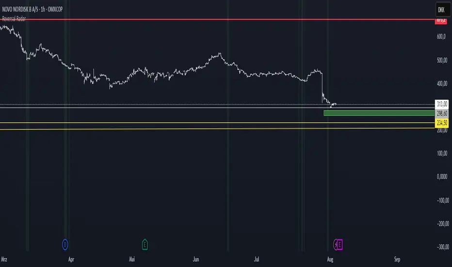
Reversal Radar
**Reversal Radar - Multi-Indicator Confirmation System**
This script combines five proven technical analysis methods into a unified reversal signal, reducing false signals through multi-indicator confirmation.
**INDICATORS USED:**
1. ADX/Directional Movement System
Determines trend direction via +DI and -DI comparison. Signal only during downtrend condition (DI- > DI+). Filters out sideways markets.
2. Custom Linear Regression Momentum
Proprietary momentum calculation based on linear regression. Measures price deviation from Keltner Channel midline. Signal on negative but rising momentum (beginning trend reversal).
3. Williams VIX Fix (WVF)
Identifies panic-selling phases. Calculates relative distance to recent high. Signal when exceeding Bollinger Bands or historical percentiles.
4. RSI Oversold Filter
Default RSI < 35 (adjustable 30-40). Filters only oversold zones for reversal setups.
5. MACD Confirmation
Signal only when MACD below zero line and below signal line. Confirms ongoing weakness before potential reversal.
**FUNCTIONALITY:**
The system generates a BUY signal only when ALL activated filters are simultaneously met. Each indicator can be individually enabled/disabled. Flexible parameter adjustment for different markets/timeframes. Reduces false signals through multi-confirmation.
**APPLICATION:**
Suitable for swing trading on higher timeframes (4H, Daily), reversal strategies in oversold markets, and combination with additional confirmation indicators.
Setup: Activate desired filters, adjust parameters to market/timeframe, check BUY signal as entry opportunity. Additional confirmation through volume/support recommended.
**INNOVATION:**
The Custom Linear Regression Momentum is a proprietary development combining Keltner Channel logic with linear regression for more precise momentum detection than standard oscillators.
**DISCLAIMER:**
This tool serves as technical analysis support. No signal should be traded without additional confirmation and risk management.
Drawdown Distribution Analysis (DDA) ACADEMIC FOUNDATION AND RESEARCH BACKGROUND
The Drawdown Distribution Analysis indicator implements quantitative risk management principles, drawing upon decades of academic research in portfolio theory, behavioral finance, and statistical risk modeling. This tool provides risk assessment capabilities for traders and portfolio managers seeking to understand their current position within historical drawdown patterns.
The theoretical foundation of this indicator rests on modern portfolio theory as established by Markowitz (1952), who introduced the fundamental concepts of risk-return optimization that continue to underpin contemporary portfolio management. Sharpe (1966) later expanded this framework by developing risk-adjusted performance measures, most notably the Sharpe ratio, which remains a cornerstone of performance evaluation in financial markets.
The specific focus on drawdown analysis builds upon the work of Chekhlov, Uryasev and Zabarankin (2005), who provided the mathematical framework for incorporating drawdown measures into portfolio optimization. Their research demonstrated that traditional mean-variance optimization often fails to capture the full risk profile of investment strategies, particularly regarding sequential losses. More recent work by Goldberg and Mahmoud (2017) has brought these theoretical concepts into practical application within institutional risk management frameworks.
Value at Risk methodology, as comprehensively outlined by Jorion (2007), provides the statistical foundation for the risk measurement components of this indicator. The coherent risk measures framework developed by Artzner et al. (1999) ensures that the risk metrics employed satisfy the mathematical properties required for sound risk management decisions. Additionally, the focus on downside risk follows the framework established by Sortino and Price (1994), while the drawdown-adjusted performance measures implement concepts introduced by Young (1991).
MATHEMATICAL METHODOLOGY
The core calculation methodology centers on a peak-tracking algorithm that continuously monitors the maximum price level achieved and calculates the percentage decline from this peak. The drawdown at any time t is defined as DD(t) = (P(t) - Peak(t)) / Peak(t) × 100, where P(t) represents the asset price at time t and Peak(t) represents the running maximum price observed up to time t.
Statistical distribution analysis forms the analytical backbone of the indicator. The system calculates key percentiles using the ta.percentile_nearest_rank() function to establish the 5th, 10th, 25th, 50th, 75th, 90th, and 95th percentiles of the historical drawdown distribution. This approach provides a complete picture of how the current drawdown compares to historical patterns.
Statistical significance assessment employs standard deviation bands at one, two, and three standard deviations from the mean, following the conventional approach where the upper band equals μ + nσ and the lower band equals μ - nσ. The Z-score calculation, defined as Z = (DD - μ) / σ, enables the identification of statistically extreme events, with thresholds set at |Z| > 2.5 for extreme drawdowns and |Z| > 3.0 for severe drawdowns, corresponding to confidence levels exceeding 99.4% and 99.7% respectively.
ADVANCED RISK METRICS
The indicator incorporates several risk-adjusted performance measures that extend beyond basic drawdown analysis. The Sharpe ratio calculation follows the standard formula Sharpe = (R - Rf) / σ, where R represents the annualized return, Rf represents the risk-free rate, and σ represents the annualized volatility. The system supports dynamic sourcing of the risk-free rate from the US 10-year Treasury yield or allows for manual specification.
The Sortino ratio addresses the limitation of the Sharpe ratio by focusing exclusively on downside risk, calculated as Sortino = (R - Rf) / σd, where σd represents the downside deviation computed using only negative returns. This measure provides a more accurate assessment of risk-adjusted performance for strategies that exhibit asymmetric return distributions.
The Calmar ratio, defined as Annual Return divided by the absolute value of Maximum Drawdown, offers a direct measure of return per unit of drawdown risk. This metric proves particularly valuable for comparing strategies or assets with different risk profiles, as it directly relates performance to the maximum historical loss experienced.
Value at Risk calculations provide quantitative estimates of potential losses at specified confidence levels. The 95% VaR corresponds to the 5th percentile of the drawdown distribution, while the 99% VaR corresponds to the 1st percentile. Conditional VaR, also known as Expected Shortfall, estimates the average loss in the worst 5% of scenarios, providing insight into tail risk that standard VaR measures may not capture.
To enable fair comparison across assets with different volatility characteristics, the indicator calculates volatility-adjusted drawdowns using the formula Adjusted DD = Raw DD / (Volatility / 20%). This normalization allows for meaningful comparison between high-volatility assets like cryptocurrencies and lower-volatility instruments like government bonds.
The Risk Efficiency Score represents a composite measure ranging from 0 to 100 that combines the Sharpe ratio and current percentile rank to provide a single metric for quick asset assessment. Higher scores indicate superior risk-adjusted performance relative to historical patterns.
COLOR SCHEMES AND VISUALIZATION
The indicator implements eight distinct color themes designed to accommodate different analytical preferences and market contexts. The EdgeTools theme employs a corporate blue palette that matches the design system used throughout the edgetools.org platform, ensuring visual consistency across analytical tools.
The Gold theme specifically targets precious metals analysis with warm tones that complement gold chart analysis, while the Quant theme provides a grayscale scheme suitable for analytical environments that prioritize clarity over aesthetic appeal. The Behavioral theme incorporates psychology-based color coding, using green to represent greed-driven market conditions and red to indicate fear-driven environments.
Additional themes include Ocean, Fire, Matrix, and Arctic schemes, each designed for specific market conditions or user preferences. All themes function effectively with both dark and light mode trading platforms, ensuring accessibility across different user interface configurations.
PRACTICAL APPLICATIONS
Asset allocation and portfolio construction represent primary use cases for this analytical framework. When comparing multiple assets such as Bitcoin, gold, and the S&P 500, traders can examine Risk Efficiency Scores to identify instruments offering superior risk-adjusted performance. The 95% VaR provides worst-case scenario comparisons, while volatility-adjusted drawdowns enable fair comparison despite varying volatility profiles.
The practical decision framework suggests that assets with Risk Efficiency Scores above 70 may be suitable for aggressive portfolio allocations, scores between 40 and 70 indicate moderate allocation potential, and scores below 40 suggest defensive positioning or avoidance. These thresholds should be adjusted based on individual risk tolerance and market conditions.
Risk management and position sizing applications utilize the current percentile rank to guide allocation decisions. When the current drawdown ranks above the 75th percentile of historical data, indicating that current conditions are better than 75% of historical periods, position increases may be warranted. Conversely, when percentile rankings fall below the 25th percentile, indicating elevated risk conditions, position reductions become advisable.
Institutional portfolio monitoring applications include hedge fund risk dashboard implementations where multiple strategies can be monitored simultaneously. Sharpe ratio tracking identifies deteriorating risk-adjusted performance across strategies, VaR monitoring ensures portfolios remain within established risk limits, and drawdown duration tracking provides valuable information for investor reporting requirements.
Market timing applications combine the statistical analysis with trend identification techniques. Strong buy signals may emerge when risk levels register as "Low" in conjunction with established uptrends, while extreme risk levels combined with downtrends may indicate exit or hedging opportunities. Z-scores exceeding 3.0 often signal statistically oversold conditions that may precede trend reversals.
STATISTICAL SIGNIFICANCE AND VALIDATION
The indicator provides 95% confidence intervals around current drawdown levels using the standard formula CI = μ ± 1.96σ. This statistical framework enables users to assess whether current conditions fall within normal market variation or represent statistically significant departures from historical patterns.
Risk level classification employs a dynamic assessment system based on percentile ranking within the historical distribution. Low risk designation applies when current drawdowns perform better than 50% of historical data, moderate risk encompasses the 25th to 50th percentile range, high risk covers the 10th to 25th percentile range, and extreme risk applies to the worst 10% of historical drawdowns.
Sample size considerations play a crucial role in statistical reliability. For daily data, the system requires a minimum of 252 trading days (approximately one year) but performs better with 500 or more observations. Weekly data analysis benefits from at least 104 weeks (two years) of history, while monthly data requires a minimum of 60 months (five years) for reliable statistical inference.
IMPLEMENTATION BEST PRACTICES
Parameter optimization should consider the specific characteristics of different asset classes. Equity analysis typically benefits from 500-day lookback periods with 21-day smoothing, while cryptocurrency analysis may employ 365-day lookback periods with 14-day smoothing to account for higher volatility patterns. Fixed income analysis often requires longer lookback periods of 756 days with 34-day smoothing to capture the lower volatility environment.
Multi-timeframe analysis provides hierarchical risk assessment capabilities. Daily timeframe analysis supports tactical risk management decisions, weekly analysis informs strategic positioning choices, and monthly analysis guides long-term allocation decisions. This hierarchical approach ensures that risk assessment occurs at appropriate temporal scales for different investment objectives.
Integration with complementary indicators enhances the analytical framework. Trend indicators such as RSI and moving averages provide directional bias context, volume analysis helps confirm the severity of drawdown conditions, and volatility measures like VIX or ATR assist in market regime identification.
ALERT SYSTEM AND AUTOMATION
The automated alert system monitors five distinct categories of risk events. Risk level changes trigger notifications when drawdowns move between risk categories, enabling proactive risk management responses. Statistical significance alerts activate when Z-scores exceed established threshold levels of 2.5 or 3.0 standard deviations.
New maximum drawdown alerts notify users when historical maximum levels are exceeded, indicating entry into uncharted risk territory. Poor risk efficiency alerts trigger when the composite risk efficiency score falls below 30, suggesting deteriorating risk-adjusted performance. Sharpe ratio decline alerts activate when risk-adjusted performance turns negative, indicating that returns no longer compensate for the risk undertaken.
TRADING STRATEGIES
Conservative risk parity strategies can be implemented by monitoring Risk Efficiency Scores across a diversified asset portfolio. Monthly rebalancing maintains equal risk contribution from each asset, with allocation reductions triggered when risk levels reach "High" status and complete exits executed when "Extreme" risk levels emerge. This approach typically results in lower overall portfolio volatility, improved risk-adjusted returns, and reduced maximum drawdown periods.
Tactical asset rotation strategies compare Risk Efficiency Scores across different asset classes to guide allocation decisions. Assets with scores exceeding 60 receive overweight allocations, while assets scoring below 40 receive underweight positions. Percentile rankings provide timing guidance for allocation adjustments, creating a systematic approach to asset allocation that responds to changing risk-return profiles.
Market timing strategies with statistical edges can be constructed by entering positions when Z-scores fall below -2.5, indicating statistically oversold conditions, and scaling out when Z-scores exceed 2.5, suggesting overbought conditions. The 95% VaR serves as a stop-loss reference point, while trend confirmation indicators provide additional validation for position entry and exit decisions.
LIMITATIONS AND CONSIDERATIONS
Several statistical limitations affect the interpretation and application of these risk measures. Historical bias represents a fundamental challenge, as past drawdown patterns may not accurately predict future risk characteristics, particularly during structural market changes or regime shifts. Sample dependence means that results can be sensitive to the selected lookback period, with shorter periods providing more responsive but potentially less stable estimates.
Market regime changes can significantly alter the statistical parameters underlying the analysis. During periods of structural market evolution, historical distributions may provide poor guidance for future expectations. Additionally, many financial assets exhibit return distributions with fat tails that deviate from normal distribution assumptions, potentially leading to underestimation of extreme event probabilities.
Practical limitations include execution risk, where theoretical signals may not translate directly into actual trading results due to factors such as slippage, timing delays, and market impact. Liquidity constraints mean that risk metrics assume perfect liquidity, which may not hold during stressed market conditions when risk management becomes most critical.
Transaction costs are not incorporated into risk-adjusted return calculations, potentially overstating the attractiveness of strategies that require frequent trading. Behavioral factors represent another limitation, as human psychology may override statistical signals, particularly during periods of extreme market stress when disciplined risk management becomes most challenging.
TECHNICAL IMPLEMENTATION
Performance optimization ensures reliable operation across different market conditions and timeframes. All technical analysis functions are extracted from conditional statements to maintain Pine Script compliance and ensure consistent execution. Memory efficiency is achieved through optimized variable scoping and array usage, while computational speed benefits from vectorized calculations where possible.
Data quality requirements include clean price data without gaps or errors that could distort distribution analysis. Sufficient historical data is essential, with a minimum of 100 bars required and 500 or more preferred for reliable statistical inference. Time alignment across related assets ensures meaningful comparison when conducting multi-asset analysis.
The configuration parameters are organized into logical groups to enhance usability. Core settings include the Distribution Analysis Period (100-2000 bars), Drawdown Smoothing Period (1-50 bars), and Price Source selection. Advanced metrics settings control risk-free rate sourcing, either from live market data or fixed rate specification, along with toggles for various risk-adjusted metric calculations.
Display options provide flexibility in visual presentation, including color theme selection from eight available schemes, automatic dark mode optimization, and control over table display, position lines, percentile bands, and standard deviation overlays. These options ensure that the indicator can be adapted to different analytical workflows and visual preferences.
CONCLUSION
The Drawdown Distribution Analysis indicator provides risk management tools for traders seeking to understand their current position within historical risk patterns. By combining established statistical methodology with practical usability features, the tool enables evidence-based risk assessment and portfolio optimization decisions.
The implementation draws upon established academic research while providing practical features that address real-world trading requirements. Dynamic risk-free rate integration ensures accurate risk-adjusted performance calculations, while multiple color schemes accommodate different analytical preferences and use cases.
Academic compliance is maintained through transparent methodology and acknowledgment of limitations. The tool implements peer-reviewed statistical techniques while clearly communicating the constraints and assumptions underlying the analysis. This approach ensures that users can make informed decisions about the appropriate application of the risk assessment framework within their broader trading and investment processes.
BIBLIOGRAPHY
Artzner, P., Delbaen, F., Eber, J.M. and Heath, D. (1999) 'Coherent Measures of Risk', Mathematical Finance, 9(3), pp. 203-228.
Chekhlov, A., Uryasev, S. and Zabarankin, M. (2005) 'Drawdown Measure in Portfolio Optimization', International Journal of Theoretical and Applied Finance, 8(1), pp. 13-58.
Goldberg, L.R. and Mahmoud, O. (2017) 'Drawdown: From Practice to Theory and Back Again', Journal of Risk Management in Financial Institutions, 10(2), pp. 140-152.
Jorion, P. (2007) Value at Risk: The New Benchmark for Managing Financial Risk. 3rd edn. New York: McGraw-Hill.
Markowitz, H. (1952) 'Portfolio Selection', Journal of Finance, 7(1), pp. 77-91.
Sharpe, W.F. (1966) 'Mutual Fund Performance', Journal of Business, 39(1), pp. 119-138.
Sortino, F.A. and Price, L.N. (1994) 'Performance Measurement in a Downside Risk Framework', Journal of Investing, 3(3), pp. 59-64.
Young, T.W. (1991) 'Calmar Ratio: A Smoother Tool', Futures, 20(1), pp. 40-42.

Ultimate Global Trading Hours📊 Global Markets Pro - Summary
What it does:
Shows real-time trading hours for 11 major stock markets worldwide
Displays countdown timers for when each market opens/closes
Includes Forex sessions and US extended hours (pre-market/after-hours)
Features advanced market sentiment analysis with Fear/Greed indicators
Key Features:
✅ Chronological market order (Sydney → Tokyo → London → NYSE, etc.)
✅ Customisable times for each market in HH:MM format
✅ Multi-factor sentiment (VIX, Bonds vs Stocks, Weekly trends, Volume)
✅ Clean interface with emoji indicators and colour coding
✅ Your timezone display with GMT+/- options
Perfect for:
Day traders tracking global market sessions
Swing traders gauging market sentiment
Anyone wanting to know when major markets are active
Result: One comprehensive dashboard showing when to trade and market mood across all time zones!

IV PercentileIV Percentile Indicator - Brief Description
What It Does
The IV Percentile Indicator measures where current implied volatility ranks compared to the past year, showing what percentage of time volatility was lower than today's level.
How It Works
Data Collection:
Tracks implied volatility (or historical volatility as proxy) for each trading day
Stores the last 252 days (1 year) of volatility readings
Uses VIX data for SPY/SPX, historical volatility for other stocks
Calculation:
IV Percentile = (Days with IV below current level) ÷ (Total days) × 100
Example: If IV Percentile = 75%, it means current volatility is higher than 75% of the past year's readings.
Visual Output
Main Display:
Blue line showing percentile (0-100%)
Reference lines at key levels (20%, 30%, 50%, 70%, 80%)
Color-coded backgrounds for quick identification
Info table with current readings
Key Levels:
80%+ (Red): Very high IV → Sell premium
70-79% (Orange): High IV → Consider selling
30-20% (Green): Low IV → Consider buying
<20% (Bright Green): Very low IV → Buy premium
Trading Application
When IV Percentile is HIGH (70%+):
Options are expensive relative to recent history
Good time to sell premium (iron condors, credit spreads)
Expect volatility to decrease toward normal levels
When IV Percentile is LOW (30%-):
Options are cheap relative to recent history
Good time to buy premium (straddles, long options)
Expect volatility to increase from compressed levels
Core Logic
The indicator helps answer: "Is this a good time to buy or sell options based on how expensive/cheap they are compared to recent history?" It removes the guesswork from volatility timing by providing historical context for current option prices.

ATR Trailing Stop with ATR Targets [v6]What the Indicator Does
This custom TradingView indicator is designed for active traders who want to automate and visualize their trailing stop management and target setting, using true market volatility. It combines the Average True Range (ATR) with dynamic market structure logic to:
Trail a stop-loss behind major swings in real time, using 2×ATR (adjustable) from the highest high in uptrends or the lowest low in downtrends.
Flip trading bias between bullish and bearish when the stop is breached.
Identify and plot three profit targets (at 1, 2, and 3 ATR from the breakout/flip point) after every stop-flip, helping traders scale out or set take-profits objectively.
Maintain a visible presence on your chart every bar to avoid indicator errors, with color and labeling for clear distinction between long/short phases.
How the Indicator Works
1. ATR Calculation
ATR Period and Multiplier: You select your preferred ATR length (default is 14 bars) and a multiplier (default is 2.0).
Volatility Adjustment: ATR measures the average "true" bar range, so the trailing stop and targets adapt to current volatility.
2. Trailing Stop Logic
Uptrend (bullish bias): The indicator tracks the highest high made since the last bearish-to-bullish flip and sets the stop at - .
The stop only raises (never lowers) during an uptrend, protecting gains in strong moves.
Downtrend (bearish bias): Tracks the lowest low made since the last bullish-to-bearish flip, with stop at + .
The stop only lowers (never raises) in a downtrend.
Flip Point: If price closes through the trailing stop, the current bias “flips,” and the logic reverses (bullish to bearish or vice versa). At the new close, flip price and bar index are stored for target calculation.
3. ATR Targets after Flip
After each stop flip:
Three targets—based on the new close price—are calculated and plotted:
Long flip (new bull bias): Target1 = close + 1×ATR, Target2 = close + 2×ATR, Target3 = close + 3×ATR.
Short flip (new bear bias): Target1 = close - 1×ATR, Target2 = close - 2×ATR, Target3 = close - 3×ATR.
These targets help with scaling out, partial profit-taking, or setting automated orders.
4. Visual Feedback
Trailing stop line: Green for long bias, red for short bias.
Targets: Distinct color-coded circles at 1, 2, 3 ATR levels from the most recent flip.
Flip Labels: Mark the bar and price where bias flipped (“Long Flip” or “Short Flip”) for quick pattern recognition.
Subtle background shading: Ensures TradingView's requirement for “indicator output every bar.”
How to Use This Indicator
Parameter Setup
ATR Period and Multiplier: Adjust to match the timeframe and volatility of your instrument.
Lower periods/multipliers for short-term/volatile trading.
Higher values for smoother signals or higher timeframes.
Starting Trend: Set to match the expected initial bias if the instrument has strong trend characteristics.
Trading Application
1. Daily Bias Approach
Establish your bias in line with your trading plan (e.g., only trade long if price is above the previous day's high, short below the previous day's low).
Only look for trades in the indicator's current bias direction, as expressed by the stop and background color.
2. Entry
Use the indicator as a real-time confirmation or trailing stop for your entries.
Breakout: Enter when price establishes the current bias, using the trailing stop as your risk level.
Reversal: Wait for a bias flip after an extended move; enter in the direction of the new bias.
VWAP Rebound: Combine with a VWAP bounce—enter only if the indicator bias supports your direction.
3. Exits/Targets
Trailing stop management: Move your stop according to the plotted line; exit if your stop is hit.
Profit-taking: Scale out or take profits as price approaches each ATR-based target.
Use the dynamic labeling to identify reversal flips and reset your plan if stopped or the bias changes.
4. Market Context
Filter and frame setups by watching correlated indicators (DXY, VIX, AUDJPY, put/call ratio) and upcoming news; trade only in the daily bias direction for best consistency.
5. Practical Tips
Combine this indicator with your custom watchlist and alert settings to get notified on flips or targets.
Review the last label ("Long Flip"/"Short Flip") and targets to plan partial exits.
Remember: ATR adapts to volatility, so the stop and targets stay proportionate even when price action shifts.
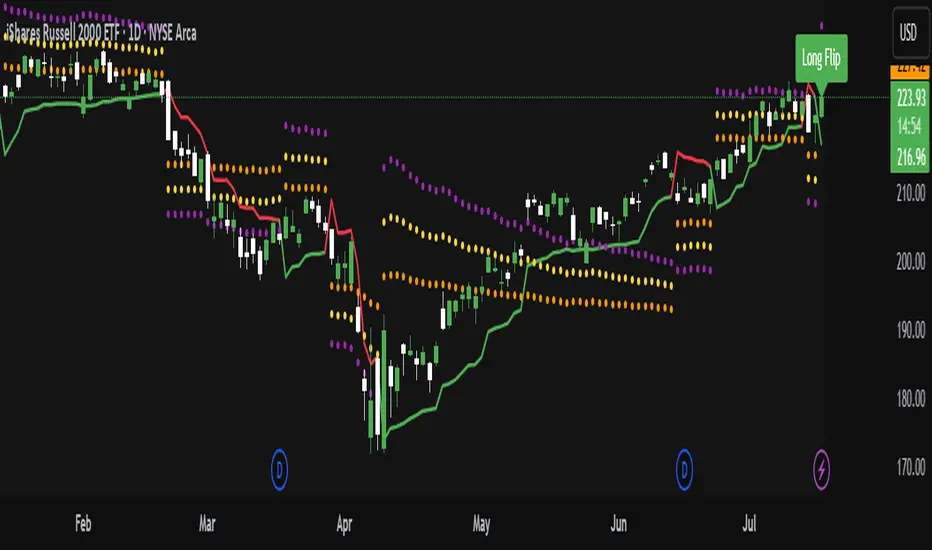
RSI Multi-Frame Multi-Asset
✅ Key Features:
Multi-Asset: Simultaneously analyze Bitcoin, SP500, Nasdaq, DXY, Gold, Oil, VIX and more
Multi-Timeframe: Configure any timeframe for all RSI calculations
Smart Average RSI: Automatically calculates the mean of all active RSI values
Special Data: Includes Bitcoin Hashrate, 10Y-2Y Spread, and US Interest Rates
Built-in Alerts: Automatic notifications on overbought/oversold crossovers
🎯 Why is it Unique?
Instead of looking at 10 different charts, you get an instant macro view of the market. The average RSI shows you the overall strength/weakness of global markets, while individual RSI values let you identify divergences and specific opportunities.
🚀 Perfect For:
Traders seeking correlations between assets
Global markets macro analysis
Identifying divergences between Bitcoin and traditional markets
Multi-timeframe breakout trading

National Financial Conditions Index (NFCI)This is one of the most important macro indicators in my trading arsenal due to its reliability across different market regimes. I'm excited to share this with the TradingView community because this Federal Reserve data is not only completely free but extraordinarily useful for portfolio management and risk assessment.
**Important Disclaimers**: Be aware that some NFCI components are updated only monthly but carry significant weighting in the composite index. Additionally, the Fed occasionally revises historical NFCI data, so historical backtests should be interpreted with some caution. Nevertheless, this remains a crucial leading indicator for financial stress conditions.
---
## What is the National Financial Conditions Index?
The National Financial Conditions Index (NFCI) is a comprehensive measure of financial stress and liquidity conditions developed by the Federal Reserve Bank of Chicago. This indicator synthesizes over 100 financial market variables into a single, interpretable metric that captures the overall state of financial conditions in the United States (Brave & Butters, 2011).
**Key Principle**: When the NFCI is positive, financial conditions are tighter than average; when negative, conditions are looser than average. Values above +1.0 historically coincide with financial crises, while values below -1.0 often signal bubble-like conditions.
## Scientific Foundation & Research
The NFCI methodology is grounded in extensive academic research:
### Core Research Foundation
- **Brave, S., & Butters, R. A. (2011)**. "Monitoring financial stability: A financial conditions index approach." *Economic Perspectives*, 35(1), 22-43.
- **Hatzius, J., Hooper, P., Mishkin, F. S., Schoenholtz, K. L., & Watson, M. W. (2010)**. "Financial conditions indexes: A fresh look after the financial crisis." *US Monetary Policy Forum Report*, No. 23.
- **Kliesen, K. L., Owyang, M. T., & Vermann, E. K. (2012)**. "Disentangling diverse measures: A survey of financial stress indexes." *Federal Reserve Bank of St. Louis Review*, 94(5), 369-397.
### Methodological Validation
The NFCI employs Principal Component Analysis (PCA) to extract common factors from financial market data, following the methodology established by **English, W. B., Tsatsaronis, K., & Zoli, E. (2005)** in "Assessing the predictive power of measures of financial conditions for macroeconomic variables." The index has been validated through extensive academic research (Koop & Korobilis, 2014).
## NFCI Components Explained
This indicator provides access to all five official NFCI variants:
### 1. **Main NFCI**
The primary composite index incorporating all financial market sectors. This serves as the main signal for portfolio allocation decisions.
### 2. **Adjusted NFCI (ANFCI)**
Removes the influence of credit market disruptions to focus on non-credit financial stress. Particularly useful during banking crises when credit markets may be impaired but other financial conditions remain stable.
### 3. **Credit Sub-Index**
Isolates credit market conditions including corporate bond spreads, commercial paper rates, and bank lending standards. Important for assessing corporate financing stress.
### 4. **Leverage Sub-Index**
Measures systemic leverage through margin requirements, dealer financing, and institutional leverage metrics. Useful for identifying leverage-driven market stress.
### 5. **Risk Sub-Index**
Captures market-based risk measures including volatility, correlation, and tail risk indicators. Provides indication of risk appetite shifts.
## Practical Trading Applications
### Portfolio Allocation Framework
Based on the academic research, the NFCI can be used for portfolio positioning:
**Risk-On Positioning (NFCI declining):**
- Consider increasing equity exposure
- Reduce defensive positions
- Evaluate growth-oriented sectors
**Risk-Off Positioning (NFCI rising):**
- Consider reducing equity exposure
- Increase defensive positioning
- Favor large-cap, dividend-paying stocks
### Academic Validation
According to **Oet, M. V., Eiben, R., Bianco, T., Gramlich, D., & Ong, S. J. (2011)** in "The financial stress index: Identification of systemic risk conditions," financial conditions indices like the NFCI provide early warning capabilities for systemic risk conditions.
**Illing, M., & Liu, Y. (2006)** demonstrated in "Measuring financial stress in a developed country: An application to Canada" that composite financial stress measures can be useful for predicting economic downturns.
## Advanced Features of This Implementation
### Dynamic Background Coloring
- **Green backgrounds**: Risk-On conditions - potentially favorable for equity investment
- **Red backgrounds**: Risk-Off conditions - time for defensive positioning
- **Intensity varies**: Based on deviation from trend for nuanced risk assessment
### Professional Dashboard
Real-time analytics table showing:
- Current NFCI level and interpretation (TIGHT/LOOSE/NEUTRAL)
- Individual sub-index readings
- Change analysis
- Portfolio guidance (Risk On/Risk Off)
### Alert System
Professional-grade alerts for:
- Risk regime changes
- Extreme stress conditions (NFCI > 1.0)
- Bubble risk warnings (NFCI < -1.0)
- Major trend reversals
## Optimal Usage Guidelines
### Best Timeframes
- **Daily charts**: Recommended for intermediate-term positioning
- **Weekly charts**: Suitable for longer-term portfolio allocation
- **Intraday**: Less effective due to weekly update frequency
### Complementary Indicators
For enhanced analysis, combine NFCI signals with:
- **VIX levels**: Confirm stress readings
- **Credit spreads**: Validate credit sub-index signals
- **Moving averages**: Determine overall market trend context
- **Economic surprise indices**: Gauge fundamental backdrop
### Position Sizing Considerations
- **Extreme readings** (|NFCI| > 1.0): Consider higher conviction positioning
- **Moderate readings** (|NFCI| 0.3-1.0): Standard position sizing
- **Neutral readings** (|NFCI| < 0.3): Consider reduced conviction
## Important Limitations & Considerations
### Data Frequency Issues
**Critical Warning**: While the main NFCI updates weekly (typically Wednesdays), some underlying components update monthly. Corporate bond indices and commercial paper rates, which carry significant weight, may cause delayed reactions to current market conditions.
**Component Update Schedule:**
- **Weekly Updates**: Main NFCI composite, most equity volatility measures
- **Monthly Updates**: Corporate bond spreads, commercial paper rates
- **Quarterly Updates**: Banking sector surveys
- **Impact**: Significant portion of index weight may lag current conditions
### Historical Revisions
The Federal Reserve occasionally revises NFCI historical data as new information becomes available or methodologies are refined. This means backtesting results should be interpreted cautiously, and the indicator works best for forward-looking analysis rather than precise historical replication.
### Market Regime Dependency
The NFCI effectiveness may vary across different market regimes. During extended sideways markets or regime transitions, signals may be less reliable. Consider combining with trend-following indicators for optimal results.
**Bottom Line**: Use NFCI for medium-term portfolio positioning guidance. Trust the directional signals while remaining aware of data revision risks and update frequency limitations. This indicator is particularly valuable during periods of financial stress when reliable guidance is most needed.
---
**Data Source**: Federal Reserve Bank of Chicago
**Update Frequency**: Weekly (typically Wednesdays)
**Historical Coverage**: 1973-present
**Cost**: Free (public Fed data)
*This indicator is for educational and analytical purposes. Always conduct your own research and risk assessment before making investment decisions.*
## References
Brave, S., & Butters, R. A. (2011). Monitoring financial stability: A financial conditions index approach. *Economic Perspectives*, 35(1), 22-43.
English, W. B., Tsatsaronis, K., & Zoli, E. (2005). Assessing the predictive power of measures of financial conditions for macroeconomic variables. *BIS Papers*, 22, 228-252.
Hatzius, J., Hooper, P., Mishkin, F. S., Schoenholtz, K. L., & Watson, M. W. (2010). Financial conditions indexes: A fresh look after the financial crisis. *US Monetary Policy Forum Report*, No. 23.
Illing, M., & Liu, Y. (2006). Measuring financial stress in a developed country: An application to Canada. *Bank of Canada Working Paper*, 2006-02.
Kliesen, K. L., Owyang, M. T., & Vermann, E. K. (2012). Disentangling diverse measures: A survey of financial stress indexes. *Federal Reserve Bank of St. Louis Review*, 94(5), 369-397.
Koop, G., & Korobilis, D. (2014). A new index of financial conditions. *European Economic Review*, 71, 101-116.
Oet, M. V., Eiben, R., Bianco, T., Gramlich, D., & Ong, S. J. (2011). The financial stress index: Identification of systemic risk conditions. *Federal Reserve Bank of Cleveland Working Paper*, 11-30.
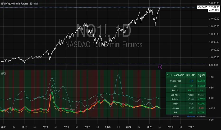
WVAD with Gap Compensation**Indicator Name:** WVAD with Gap Compensation
**Purpose:** Enhances the classic Williams Vix Fix (WVAD) by incorporating the impact of price gaps (jump ups/downs) in its calculation.
**Key Features:**
1. **Gap Detection:** Automatically identifies significant gaps (default: >0.5% from prior bar's high/low).
2. **Gap Compensation:** Adjusts the WVAD calculation by adding the gap size to the daily price change.
3. **Dynamic Weighting:** Applies a multiplier (1.2x or 1.5x) to the WVAD value on days with medium/large gaps (based on ATR).
4. **Visualization:**
- Plots the enhanced WVAD line (blue) and optionally the original WVAD (gray circles).
- Marks gap events with colored arrows (green ▲ for gap up, red ▼ for gap down) and connects the gap's impact with dashed lines.
- Includes a zero line for reference.
**Use Cases:**
- Gauges the true strength of money flow by accounting for gaps.
- Identifies potential trend shifts around gap events.
- Filters noise by focusing on significant gaps.
**Parameters:**
- `Accumulation Period`: Number of days to sum WVAD (default: 12).
- `Gap Threshold (%)`: Minimum gap size to trigger compensation (default: 0.5%).
- `Show Original WVAD`: Toggles display of the classic WVAD.
**Version:** Pine Script® v6

Fear and Greed Index [DunesIsland]The Fear and Greed Index is a sentiment indicator designed to measure the emotions driving the stock market, specifically investor fear and greed. Fear represents pessimism and caution, while greed reflects optimism and risk-taking. This indicator aggregates multiple market metrics to provide a comprehensive view of market sentiment, helping traders and investors gauge whether the market is overly fearful or excessively greedy.How It WorksThe Fear and Greed Index is calculated using four key market indicators, each capturing a different aspect of market sentiment:
Market Momentum (30% weight)
Measures how the S&P 500 (SPX) is performing relative to its 125-day simple moving average (SMA).
A higher value indicates that the market is trading well above its moving average, signaling greed.
Stock Price Strength (20% weight)
Calculates the net number of stocks hitting 52-week highs minus those hitting 52-week lows on the NYSE.
A greater number of net highs suggests strong market breadth and greed.
Put/Call Options (30% weight)
Uses the 5-day average of the put/call ratio.
A lower ratio (more call options being bought) indicates greed, as investors are betting on rising prices.
Market Volatility (20% weight)
Utilizes the VIX index, which measures market volatility.
Lower volatility is associated with greed, as investors are less fearful of large market swings.
Each component is normalized using a z-score over a 252-day lookback period (approximately one trading year) and scaled to a range of 0 to 100. The final Fear and Greed Index is a weighted average of these four components, with the weights specified above.Key FeaturesIndex Range: The index value ranges from 0 to 100:
0–25: Extreme Fear (red)
25–50: Fear (orange)
50–75: Neutral (yellow)
75–100: Greed (green)
Dynamic Plot Color: The plot line changes color based on the index value, visually indicating the current sentiment zone.
Reference Lines: Horizontal lines are plotted at 0, 25, 50, 75, and 100 to represent the different sentiment levels: Extreme Fear, Fear, Neutral, Greed, and Extreme Greed.
How to Interpret
Low Values (0–25): Indicate extreme fear, which may suggest that the market is oversold and could be due for a rebound.
High Values (75–100): Indicate greed, which may signal that the market is overbought and could be at risk of a correction.
Neutral Range (25–75): Suggests a balanced market sentiment, neither overly fearful nor greedy.
This indicator is a valuable tool for contrarian investors, as extreme readings often precede market reversals. However, it should be used in conjunction with other technical and fundamental analysis tools for a well-rounded view of the market.
Ticker Pulse Meter + Fear EKG StrategyDescription
The Ticker Pulse Meter + Fear EKG Strategy is a technical analysis tool designed to identify potential entry and exit points for long positions based on price action relative to historical ranges. It combines two proprietary indicators: the Ticker Pulse Meter (TPM), which measures price positioning within short- and long-term ranges, and the Fear EKG, a VIX-inspired oscillator that detects extreme market conditions. The strategy is non-repainting, ensuring signals are generated only on confirmed bars to avoid false positives. Visual enhancements, such as optional moving averages and Bollinger Bands, provide additional context but are not core to the strategy's logic. This script is suitable for traders seeking a systematic approach to capturing momentum and mean-reversion opportunities.
How It Works
The strategy evaluates price action using two key metrics:
Ticker Pulse Meter (TPM): Measures the current price's position within short- and long-term price ranges to identify momentum or overextension.
Fear EKG: Detects extreme selling pressure (akin to "irrational selling") by analyzing price behavior relative to historical lows, inspired by volatility-based oscillators.
Entry signals are generated when specific conditions align, indicating potential buying opportunities. Exits are triggered based on predefined thresholds or partial position closures to manage risk. The strategy supports customizable lookback periods, thresholds, and exit percentages, allowing flexibility across different markets and timeframes. Visual cues, such as entry/exit dots and a position table, enhance usability, while optional overlays like moving averages and Bollinger Bands provide additional chart context.
Calculation Overview
Price Range Calculations:
Short-Term Range: Uses the lowest low (min_price_short) and highest high (max_price_short) over a user-defined short lookback period (lookback_short, default 50 bars).
Long-Term Range: Uses the lowest low (min_price_long) and highest high (max_price_long) over a user-defined long lookback period (lookback_long, default 200 bars).
Percentage Metrics:
pct_above_short: Percentage of the current close above the short-term range.
pct_above_long: Percentage of the current close above the long-term range.
Combined metrics (pct_above_long_above_short, pct_below_long_below_short) normalize price action for signal generation.
Signal Generation:
Long Entry (TPM): Triggered when pct_above_long_above_short crosses above a user-defined threshold (entryThresholdhigh, default 20) and pct_below_long_below_short is below a low threshold (entryThresholdlow, default 40).
Long Entry (Fear EKG): Triggered when pct_below_long_below_short crosses under an extreme threshold (orangeEntryThreshold, default 95), indicating potential oversold conditions.
Long Exit: Triggered when pct_above_long_above_short crosses under a profit-taking level (profitTake, default 95). Partial exits are supported via a user-defined percentage (exitAmt, default 50%).
Non-Repainting Logic: Signals are calculated using data from the previous bar ( ) and only plotted on confirmed bars (barstate.isconfirmed), ensuring reliability.
Visual Enhancements:
Optional moving averages (SMA, EMA, WMA, VWMA, or SMMA) and Bollinger Bands can be enabled for trend context.
A position table displays real-time metrics, including open positions, Fear EKG, and Ticker Pulse values.
Background highlights mark periods of high selling pressure.
Entry Rules
Long Entry:
TPM Signal: Occurs when the price shows strength relative to both short- and long-term ranges, as defined by pct_above_long_above_short crossing above entryThresholdhigh and pct_below_long_below_short below entryThresholdlow.
Fear EKG Signal: Triggered by extreme selling pressure, when pct_below_long_below_short crosses under orangeEntryThreshold. This signal is optional and can be toggled via enable_yellow_signals.
Entries are executed only on confirmed bars to prevent repainting.
Exit Rules
Long Exit: Triggered when pct_above_long_above_short crosses under profitTake.
Partial exits are supported, with the strategy closing a user-defined percentage of the position (exitAmt) up to four times per position (exit_count limit).
Exits can be disabled or adjusted via enable_short_signal and exitPercentage settings.
Inputs
Backtest Start Date: Defines the start of the backtesting period (default: Jan 1, 2017).
Lookback Periods: Short (lookback_short, default 50) and long (lookback_long, default 200) periods for range calculations.
Resolution: Timeframe for price data (default: Daily).
Entry/Exit Thresholds:
entryThresholdhigh (default 20): Threshold for TPM entry.
entryThresholdlow (default 40): Secondary condition for TPM entry.
orangeEntryThreshold (default 95): Threshold for Fear EKG entry.
profitTake (default 95): Exit threshold.
exitAmt (default 50%): Percentage of position to exit.
Visual Options: Toggle for moving averages and Bollinger Bands, with customizable types and lengths.
Notes
The strategy is designed to work across various timeframes and assets, with data sourced from user-selected resolutions (i_res).
Alerts are included for long entry and exit signals, facilitating integration with TradingView's alert system.
The script avoids repainting by using confirmed bar data and shifted calculations ( ).
Visual elements (e.g., SMA, Bollinger Bands) are inspired by standard Pine Script practices and are optional, not integral to the core logic.
Usage
Apply the script to a chart, adjust input settings to suit your trading style, and use the visual cues (entry/exit dots, position table) to monitor signals. Enable alerts for real-time notifications.
Designed to work best on Daily timeframe.
Movement WatcherMovement Watcher – Intraday Price Change Alert
This indicator tracks the percentage price movement of a selected symbol (e.g., VIX) from a configurable start time. If the intraday movement crosses a defined threshold (up or down), it triggers a one-time alert per day.
Key Features:
Monitors intraday % change from the specified start time.
Triggers one-time alerts for upper or lower threshold crossings.
Optional end time for monitoring period.
Visual plots and alert markers.
Useful for automated trading via webhook integrations.
This script was designed to work with automated trading tools such as the Trading Automation Toolbox. You can use it to generate alerts based on intraday volatility and route them via webhook for automated strategies.
Cycle Composite 3.6 WeightedThe Cycle Composite is a multi-factor market cycle model designed to classify long-term market behavior into distinct phases using normalized and weighted data inputs.
It combines ten key on-chain, dominance, volatility, sentiment, and trend-following metrics into a single composite output. The goal is to provide a clearer understanding of where the market may stand in the broader cycle (e.g., accumulation, early bull, late bull, or euphoria).
This version (3.4) introduces flexible weighting, trend strength markers, and additional context-aware signals such as risk-on confirmations and altseason flags.
Phases Identified:
The model categorizes the market into one of five zones:
Euphoria (> 85)
Late Bull (70 – 85)
Mid Bull (50 – 70)
Early Bull (30 – 50)
Fear (< 30)
Each phase is determined by a smoothed EMA of the weighted composite score.
Data Sources and Metrics Used (10 total):
BTC Dominance (CRYPTOCAP:BTC.D)
Stablecoin Dominance (USDT + USDC average) (inverted for risk-on)
ETH Dominance (CRYPTOCAP:ETH.D)
BBWP (normalized Bollinger Band Width % over 1-year window)
WVF (Williams VIX Fix for volatility spike detection)
NUPL (Net Unrealized Profit/Loss, external source)
CMF (Chaikin Money Flow, smoothed volume accumulation)
CEX Open Interest (custom input from DAO / external source)
Whale Inflows (custom input from whale exchange transfer data)
Google Trends Average (BTC, Crypto, Altcoin terms)
All inputs are normalized over a 200-bar window and combined via weighted averaging, where each weight is user-configurable.
Additional Features:
Phase Labels: Labels are printed only when a new phase is entered.
Bull Continuation Marker: Triangle up when composite makes higher highs and NUPL increases.
Weakening Marker: Triangle down when composite rolls over in Late Bull and NUPL falls.
Risk-On Signal: Green circle appears when CMF and Google Trends are both rising.
Altseason Flag: Orange diamond appears when dominance of "others.d" exceeds BTC.D and ETH.D and composite is above 50.
Background Shading: Each phase is shaded with a semi-transparent background color.
Timeframe-Aware Display: All markers and signals are shown only on weekly timeframe for clarity.
Intended Use:
This script is intended for educational and macro-trend analysis purposes.
It can be used to:
Identify macro cycle position (accumulation, bull phases, euphoria, etc.)
Spot long-term trend continuation or weakening signals
Add context to price action with external on-chain and sentiment data
Time rotation events such as altseason risk
Disclaimer:
This script does not constitute financial advice.
It is intended for informational and research purposes only.
Users should conduct their own due diligence and analysis before making investment decisions.
