Volume Profile Skew [BackQuant]Volume Profile Skew
Overview
Volume Profile Skew is a market-structure indicator that answers a specific question most volume profiles do not:
“Is volume concentrating toward lower prices (accumulation) or higher prices (distribution) inside the current profile range?”
A standard volume profile shows where volume traded, but it does not quantify the shape of that distribution in a single number. This script builds a volume profile over a rolling lookback window, extracts the key profile levels (POC, VAH, VAL, and a volume-weighted mean), then computes the skewness of the volume distribution across price bins. That skewness becomes an oscillator, smoothed into a regime signal and paired with visual profile plotting, key level lines, and historical POC tracking.
This gives you two layers at once:
A full profile and its important levels (where volume is).
A skew metric (how volume is leaning within that range).
What this indicator is based on
The foundation comes from classical “volume at price” concepts used in Market Profile and Volume Profile analysis:
POC (Point of Control): the price level with the highest traded volume.
Value Area (VAH/VAL): the zone containing the bulk of activity, commonly 70% of total volume.
Volume-weighted mean (VWMP in this script): the average price weighted by volume, a “center of mass” for traded activity.
Where this indicator extends the idea is by treating the volume profile as a statistical distribution across price. Once you treat “volume by price bin” as a probability distribution (weights sum to 1), you can compute distribution moments:
Mean: where the mass is centered.
Standard deviation: how spread-out it is.
Skewness: whether the distribution has a heavier tail toward higher or lower prices.
This is not a gimmick. Skewness is a standard statistic in probability theory. Here it is applied to “volume concentration across price”, not to returns.
Core concept: what “skew” means in a volume profile
Imagine a profile range from Low to High, split into bins. Each bin has some volume. You can get these shapes:
Balanced profile: volume is fairly symmetric around the mean, skew near 0.
Bottom-heavy profile: more volume at lower prices, with a tail toward higher prices, skew tends to be positive.
Top-heavy profile: more volume at higher prices, with a tail toward lower prices, skew tends to be negative.
In this script:
Positive skew is labeled as ACCUMULATION.
Negative skew is labeled as DISTRIBUTION.
Near-zero skew is NEUTRAL.
Important: accumulation here does not mean “buying will immediately pump price.” It means the profile shape suggests more participation at lower prices inside the current lookback range. Distribution means participation is heavier at higher prices.
How the volume profile is built
1) Define the analysis window
The profile is computed on a rolling window:
Lookback Period: number of bars included (capped by available history).
Profile Resolution (bins): number of price bins used to discretize the high-low range.
The script finds the highest high and lowest low in the lookback window to define the price range:
rangeHigh = highest high in window
rangeLow = lowest low in window
binSize = (rangeHigh - rangeLow) / bins
2) Create bin midpoints
Each bin gets a midpoint “price” used for calculations:
price = rangeLow + binSize * (b + 0.5)
These midpoints are what the mean, variance, and skewness are computed on.
3) Distribute each candle’s volume into bins
This is a key implementation detail. Real volume profiles require tick-level data, but Pine does not provide that. So the script approximates volume-at-price using candle ranges:
For each bar in the lookback:
Determine which bins its low-to-high range touches.
Split that candle’s total volume evenly across the touched bins.
So if a candle spans 6 bins, each bin gets volume/6 from that bar. This is a practical, consistent approximation for “where trading could have occurred” inside the bar.
This approach has tradeoffs:
It does not know where within the candle the volume truly traded.
It assumes uniform distribution across the candle range.
It becomes more meaningful with larger samples (bigger lookback) and/or higher timeframes.
But it is still useful because the purpose here is the shape of the distribution across the whole window, not exact microstructure.
Key profile levels: POC, VAH, VAL, VWMP
POC (Point of Control)
POC is found by scanning bins and selecting the bin with maximum volume. The script stores:
pocIndex: which bin has max volume
poc price: midpoint price of that bin
Value Area (VAH/VAL) using 70% volume
The script builds the value area around the POC outward until it captures 70% of total volume:
Start with the POC bin.
Expand one bin at a time to the side with more volume.
Stop when accumulated volume >= 70% of total profile volume.
Then:
VAL = rangeLow + binSize * lowerIdx
VAH = rangeLow + binSize * (upperIdx + 1)
This produces a classic “where most business happened” zone.
VWMP (Volume-Weighted Mean Price)
This is essentially the center of mass of the profile:
VWMP = sum(price * volume ) / totalVolume
It is similar in spirit to VWAP, but it is computed over the profile bins, not from bar-by-bar typical price.
Skewness calculation: turning the profile into an oscillator
This is the main feature.
1) Treat volumes as weights
For each bin:
weight = volume / totalVolume
Now weights sum to 1.
2) Compute weighted mean
Mean price:
mean = sum(weight * price )
3) Compute weighted variance and std deviation
Variance:
variance = sum(weight * (price - mean)^2)
stdDev = sqrt(variance)
4) Compute weighted third central moment
Third moment:
m3 = sum(weight * (price - mean)^3)
5) Standardize to skewness
Skewness:
rawSkew = m3 / (stdDev^3)
This standardization matters. Without it, the value would explode or shrink based on profile scale. Standardized skewness is dimensionless and comparable.
Smoothing and regime rules
Raw skewness can be jumpy because:
profile bins change as rangeHigh/rangeLow shift,
one high-volume candle can reshape the distribution,
volume regimes change quickly in crypto.
So the indicator applies EMA smoothing:
smoothedSkew = EMA(rawSkew, smooth)
Then it classifies regime using fixed thresholds:
Bullish (ACCUMULATION): smoothedSkew > +0.25
Bearish (DISTRIBUTION): smoothedSkew < -0.25
Neutral: between those values
Signals are generated on threshold cross events:
Bull signal when smoothedSkew crosses above +0.25
Bear signal when smoothedSkew crosses below -0.25
This makes the skew act like a regime oscillator rather than a constantly flipping color.
Volume Profile plotting modes
The script draws the profile on the last bar, using boxes for each bin, anchored to the right with a configurable offset. The width of each profile bar is normalized by max bin volume:
volRatio = binVol / maxVol
barWidth = volRatio * width
Three style modes exist:
1) Gradient
Uses a “jet-like” gradient based on volRatio (blue → red). Higher-volume bins stand out naturally. Transparency increases as volume decreases, so low-volume bins fade.
2) Solid
Uses the current regime color (bull/bear/neutral) for all bins, with transparency. This makes the profile read as “structure + regime.”
3) Skew Highlight
Highlights bins that match the skew bias:
If skew bullish, emphasize lower portion of profile.
If skew bearish, emphasize higher portion of profile.
Else, keep most bins neutral.
This is a visual “where the skew is coming from” mode.
Historical POC tracking and Naked POCs
This script also treats POCs as meaningful levels over time, similar to how traders track old VA levels.
What is a “naked POC”?
A “naked POC” is a previously formed POC that has not been revisited (retested) by price since it was recorded. Many traders watch these as potential reaction zones because they represent prior “maximum traded interest” that the market has not re-engaged with.
How this script records POCs
It stores a new historical POC when:
At least updatebars have passed since the last stored POC, and
The POC has changed by at least pochangethres (%) from the last stored value.
New stored POCs are flagged as naked by default.
How naked becomes tested
On each update, the script checks whether price has entered a small zone around a naked POC:
zoneSize = POC * 0.002 (about 0.2%)
If bar range overlaps that zone, mark it as tested (not naked).
Display controls:
Highlight Naked POCs: draws and labels untested POCs.
Show Tested POCs: optionally draw tested ones in a muted color.
To avoid clutter, the script limits stored POCs to the most recent 20 and avoids drawing ones too close to the current POC.
On-chart key levels and what they mean
When enabled, the script draws the current lookback profile levels on the price chart:
POC (solid): the “most traded” price.
VAH/VAL (dashed): boundaries of the 70% value area.
VWMP (dotted): volume-weighted mean of the profile distribution.
Interpretation framework (practical, not mystical):
POC often behaves like a magnet in balanced conditions.
VAH/VAL define the “accepted” area, breaks can signal auction continuation.
VWMP is a fair-value reference, useful as a mean anchor when skew is neutralizing.
Oscillator panel and histogram
The skew oscillator is plotted in a separate pane:
Line: smoothedSkew, colored by regime.
Histogram: smoothedSkew as bars, colored by sign.
Fill: subtle shading above/below 0 to reinforce bias.
This makes it easy to read:
Direction of bias (positive vs negative).
Strength (distance from 0 and from thresholds).
Transitions (crosses of ±0.25).
Info table: what it summarizes
On the last bar, a table prints key diagnostics:
Current skew value (smoothed).
Regime label (ACCUMULATION / DISTRIBUTION / NEUTRAL).
Current POC, VAH, VAL, VWMP.
Count of naked POCs still active.
A simple “volume location” hint (lower/higher/balanced).
This is designed for quick scanning without reading the entire profile.
Alerts
The indicator includes alerts for:
Skew regime shifts (cross above +0.25, cross below -0.25).
Price crossing above/below current POC.
Approaching a naked POC (within 1% of any active naked POC).
The “approaching naked POC” alert is useful as a heads-up that price is entering a historically important volume magnet/reaction zone.
How to use it properly
1) Regime filter
Use skew regime to decide what type of trades you should prioritize:
ACCUMULATION (positive skew): market activity is heavier at lower prices, pullbacks into value or below VWMP often matter more.
DISTRIBUTION (negative skew): activity is heavier at higher prices, rallies into value or above VWMP often matter more.
NEUTRAL: mean-reversion and POC magnet behavior tends to dominate.
This is not “buy when green.” It is context for what the auction is doing.
2) Level-based execution
Combine skew with VA/POC levels:
In neutral regimes, expect rotations around POC and inside VA.
In strong skew regimes, watch for acceptance away from POC and reactions at VA edges.
3) Naked POCs as targets and reaction zones
Naked POCs can act like unfinished business. Common workflows:
As targets in rotations.
As areas to reduce risk when price is approaching.
As “if it breaks cleanly, trend continuation” markers when price returns with force.
Parameter tuning guidance
Lookback
Controls how “local” the profile is.
Shorter: reacts faster, more sensitive to recent moves.
Longer: more stable, better for swing context.
Bins
Controls resolution of the profile.
Higher bins: more detail, more computation, more sensitive profile shape.
Lower bins: smoother, less detail, more stable skew.
Smoothing
Controls how noisy the skew oscillator is.
Higher smoothing: fewer regime flips, slower response.
Lower smoothing: more responsive, more false transitions.
POC tracking settings
Update interval and threshold decide how many historical POCs you store and how different they must be. If you set them too loose, you will spam levels. If too strict, you will miss meaningful shifts.
Limitations and what not to assume
This indicator uses candle-range volume distribution because Pine cannot see tick-level volume-at-price. That means:
The profile is an approximation of where volume could have traded, not exact tape data.
Skew is best treated as a structural bias, not a precise signal generator.
Extreme single-bar events can distort the distribution briefly, smoothing helps but cannot remove reality.
Summary
Volume Profile Skew takes standard volume profile structure (POC, Value Area, volume-weighted mean) and adds a statistically grounded measure of profile shape using skewness. The result is a regime oscillator that quantifies whether volume concentration is leaning toward lower prices (accumulation) or higher prices (distribution), while also plotting the full profile, key levels, and historical naked POCs for actionable context.
SKEW

LibBrStLibrary "LibBrSt"
This is a library for quantitative analysis, designed to estimate
the statistical properties of price movements *within* a single
OHLC bar, without requiring access to tick data. It provides a
suite of estimators based on various statistical and econometric
models, allowing for analysis of intra-bar volatility and
price distribution.
Key Capabilities:
1. **Price Distribution Models (`PriceEst`):** Provides a selection
of estimators that model intra-bar price action as a probability
distribution over the range. This allows for the
calculation of the intra-bar mean (`priceMean`) and standard
deviation (`priceStdDev`) in absolute price units. Models include:
- **Symmetric Models:** `uniform`, `triangular`, `arcsine`,
`betaSym`, and `t4Sym` (Student-t with fat tails).
- **Skewed Models:** `betaSkew` and `t4Skew`, which adjust
their shape based on the Open/Close position.
- **Model Assumptions:** The skewed models rely on specific
internal constants. `betaSkew` uses a fixed concentration
parameter (`BETA_SKEW_CONCENTRATION = 4.0`), and `t4Sym`/`t4Skew`
use a heuristic scaling factor (`T4_SHAPE_FACTOR`)
to map the distribution.
2. **Econometric Log-Return Estimators (`LogEst`):** Includes a set of
econometric estimators for calculating the volatility (`logStdDev`)
and drift (`logMean`) of logarithmic returns within a single bar.
These are unit-less measures. Models include:
- **Parkinson (1980):** A High-Low range estimator.
- **Garman-Klass (1980):** An OHLC-based estimator.
- **Rogers-Satchell (1991):** An OHLC estimator that accounts
for non-zero drift.
3. **Distribution Analysis (PDF/CDF):** Provides functions to work
with the Probability Density Function (`pricePdf`) and
Cumulative Distribution Function (`priceCdf`) of the
chosen price model.
- **Note on `priceCdf`:** This function uses analytical (exact)
calculations for the `uniform`, `triangular`, and `arcsine`
models. For all other models (e.g., `betaSkew`, `t4Skew`),
it uses **numerical integration (Simpson's rule)** as
an approximation of the cumulative probability.
4. **Mathematical Functions:** The library's Beta distribution
models (`betaSym`, `betaSkew`) are supported by an internal
implementation of the natural log-gamma function, which is
based on the Lanczos approximation.
---
**DISCLAIMER**
This library is provided "AS IS" and for informational and
educational purposes only. It does not constitute financial,
investment, or trading advice.
The author assumes no liability for any errors, inaccuracies,
or omissions in the code. Using this library to build
trading indicators or strategies is entirely at your own risk.
As a developer using this library, you are solely responsible
for the rigorous testing, validation, and performance of any
scripts you create based on these functions. The author shall
not be held liable for any financial losses incurred directly
or indirectly from the use of this library or any scripts
derived from it.
priceStdDev(estimator, offset)
Estimates **σ̂** (standard deviation) *in price units* for the current
bar, according to the chosen `PriceEst` distribution assumption.
Parameters:
estimator (series PriceEst) : series PriceEst Distribution assumption (see enum).
offset (int) : series int To offset the calculated bar
Returns: series float σ̂ ≥ 0 ; `na` if undefined (e.g. zero range).
priceMean(estimator, offset)
Estimates **μ̂** (mean price) for the chosen `PriceEst` within the
current bar.
Parameters:
estimator (series PriceEst) : series PriceEst Distribution assumption (see enum).
offset (int) : series int To offset the calculated bar
Returns: series float μ̂ in price units.
pricePdf(estimator, price, offset)
Probability-density under the chosen `PriceEst` model.
**Returns 0** when `p` is outside the current bar’s .
Parameters:
estimator (series PriceEst) : series PriceEst Distribution assumption (see enum).
price (float) : series float Price level to evaluate.
offset (int) : series int To offset the calculated bar
Returns: series float Density value.
priceCdf(estimator, upper, lower, steps, offset)
Cumulative probability **between** `upper` and `lower` under
the chosen `PriceEst` model. Outside-bar regions contribute zero.
Uses a fast, analytical calculation for Uniform, Triangular, and
Arcsine distributions, and defaults to numerical integration
(Simpson's rule) for more complex models.
Parameters:
estimator (series PriceEst) : series PriceEst Distribution assumption (see enum).
upper (float) : series float Upper Integration Boundary.
lower (float) : series float Lower Integration Boundary.
steps (int) : series int # of sub-intervals for numerical integration (if used).
offset (int) : series int To offset the calculated bar.
Returns: series float Probability mass ∈ .
logStdDev(estimator, offset)
Estimates **σ̂** (standard deviation) of *log-returns* for the current bar.
Parameters:
estimator (series LogEst) : series LogEst Distribution assumption (see enum).
offset (int) : series int To offset the calculated bar
Returns: series float σ̂ (unit-less); `na` if undefined.
logMean(estimator, offset)
Estimates μ̂ (mean log-return / drift) for the chosen `LogEst`.
The returned value is consistent with the assumptions of the
selected volatility estimator.
Parameters:
estimator (series LogEst) : series LogEst Distribution assumption (see enum).
offset (int) : series int To offset the calculated bar
Returns: series float μ̂ (unit-less log-return).

Implied Volatility RangeThe Implied Volatility Range is a forward-looking tool that transforms option market data into probability ranges for future prices. Based on the lognormal distribution of asset prices assumed in modern option pricing models, it converts the implied volatility curve into a volatility cone with dynamic labels that show the market’s expectations for the price distribution at a specific point in time. At the selected future date, it displays projected price levels and their percentage change from today’s close across 1, 2, and 3 standard deviation (σ) ranges:
1σ range = ~68.2% probability the price will remain within this range.
2σ range = ~95.4% probability the price will remain within this range.
3σ range = ~99.7% probability the price will remain within this range.
What makes this indicator especially useful is its ability to incorporate implied volatility skew. When only ATM IV (%) is entered, the indicator displays the standard Black–Scholes lognormal distribution. By adding High IV (%) and Low IV (%) values tied to strikes above and below the current price, the indicator interpolates between these inputs to approximate the implied volatility skew. This adjustment produces a market-implied probability distribution that indicates whether the option market is leaning bullish or bearish, based on the data entered in the menu:
ATM IV (%) = Implied volatility at the current spot price (at-the-money).
High IV (%) = Implied volatility at a strike above the current spot price.
High Strike = Strike price corresponding to the High IV input (OTM call).
Low IV (%) = Implied volatility at a strike below the current spot price.
Low Strike = Strike price corresponding to the Low IV input (OTM put).
Expiration (Day, Month, Year) = Option expiration date for the projection.
Once these inputs are entered, the indicator calculates implied probability ranges and, if both High IV and Low IV values are provided, adjusts for skew to approximate the option market’s distribution. If no implied volatility data is supplied, the indicator defaults to a lognormal distribution based on historical volatility, using past realized volatility over the same forward horizon. This keeps the tool functional even without implied volatility inputs, though in that case the output represents only an approximation of ATM IV, not the actual market view.
In summary, the Implied Volatility Range is a powerful tool that translates implied volatility inputs into a clear and practical estimate of the market’s expectations for future prices. It allows traders to visualize the probability of price ranges while also highlighting directional bias, a dimension often difficult to interpret from traditional implied volatility charts. It should be emphasized, however, that this tool reflects only the market’s expectations at a specific point in time, which may change as new information and trading activity reshape implied volatility.

Expected Range and SkewThis is an open source and updated version of my previous "Confidence Interval" script. This script provides you with the expected range over a given time period in the future and the skew of that range. For example, if you wanted to know the expected 1 standard deviation range of MSFT over the next 20 days, this will tell you that. Additionally, this script will also tell you the skew of the expected range.
How to use this script:
1) Enter the length, this will determine the number of data points used in the calculation of the expected range.
2) Enter the amount of time you want projected forward in minutes, hours, and days.
3) Input standard deviation of the expected range.
4) Pick the type of data you want shown from the dropdown menu. Your choices are either the expected range or the skew of the expected range.
5) Enter the x and y coordinates of the label (optional). This is useful so it doesn't impede your view of the plot.
Here are a few notes about this script:
First, the expected range line gives you the width of said range (upper bound - lower bound), and the label will tell you specifically what the upper and lower bounds of the expected range are.
Second, this script will work on any of the default timeframes, but you need to be careful with how far out you try to project the expected range depending on the timeframe you're using. For example, if you're using the 1min timeframe, it probably won't do you any good trying to project the expected range over the next 20 days; or if you're using the daily timeframe it doesn't make sense to try to project the expected range for the next 5 hours. You can tell if the time horizon you're trying to project doesn't work well with the chart timeframe you're using if the current price is outside of either the upper or lower bounds provided in the label. If the current price is within the upper and lower bounds provided in the label, then the time horizon that you're projecting over is reasonable for the chart timeframe you're using.
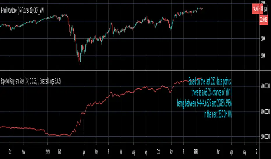
Third, this script does not countdown automatically, so the time provided in the label will stay the same. For example, in the picture above, the expected range of Dow Futures over the next 23 days from January 12th, 2021 is calculated. But when tomorrow comes it won't count down to 22 days, instead it will show the range over the next 23 days from January 13th, 2021. So if you want the time horizon to change as time goes on you will have to update this yourself manually.
Lastly, if you try to set an alert on this script, you will get a warning about it possibly repainting. This is because of the label, not the plot itself. The label constantly updates itself, which triggers the warning. I tested setting alerts on this script both with and without the inclusion of the label, and without the label the repainting warning did not occur. So remember, if you set an alert on this script you will get a warning about it possibly repainting, but this is because of the label constantly updating, not the plot itself.
Implied Volatility SuiteThis is an updated, more robust, and open source version of my 2 previous scripts : "Implied Volatility Rank & Model-Free IVR" and "IV Rank & IV Percentile".
This specific script provides you with 4 different types of volatility data: 1)Implied volatility, 2) Implied Volatility Rank, 3)Implied Volatility Percentile, 4)Skew Index.
1) Implied Volatility is the market's forecast of a likely movement, usually 1 standard deviation, in a securities price.
2) Implied Volatility Rank, ranks IV in relation to its high and low over a certain period of time. For example if over the past year IV had a high of 20% and a low of 10% and is currently 15%; the IV rank would be 50%, as 15 is 50% of the way between 10 & 20. IV Rank is mean reverting, meaning when IV Rank is high (green) it is assumed that future volatility will decrease; while if IV rank is low (red) it is assumed that future volatility will increase.
3) Implied Volatility Percentile ranks IV in relation to how many previous IV data points are less than the current value. For example if over the last 5 periods Implied volatility was 10%,12%,13%,14%,20%; and the current implied volatility is 15%, the IV percentile would be 80% as 4 out of the 5 previous IV values are below the current IV of 15%. IV Percentile is mean reverting, meaning when IV Percentile is high (green) it is assumed that future volatility will decrease; while if IV percentile is low (red) it is assumed that future volatility will increase. IV Percentile is more robust than IV Rank because, unlike IV Rank which only looks at the previous highs and lows, IV Percentile looks at all data points over the specified time period.
4)The skew index is an index I made that looks at volatility skew. Volatility Skew compares implied volatility of options with downside strikes versus upside strikes. If downside strikes have higher IV than upside strikes there is negative volatility skew. If upside strikes have higher IV than downside strikes then there is positive volatility skew. Typically, markets have a negative volatility skew, this has been the case since Black Monday in 1987. All negative skew means is that projected option contract prices tend to go down over time regardless of market conditions.
Additionally, this script provides two ways to calculate the 4 data types above: a)Model-Based and b)VixFix.
a) The Model-Based version calculates the four data types based on a model that projects future volatility. The reason that you would use this version is because it is what is most commonly used to calculate IV, IV Rank, IV Percentile, and Skew; and is closest to real world IV values. This version is what is referred to when people normally refer to IV. Additionally, the model version of IV, Rank, Percentile, and Skew are directionless.
b) The VixFix version calculates the four data types based on the VixFix calculation. The reason that you would use this version is because it is based on past price data as opposed to a model, and as such is more sensitive to price action. Additionally, because the VixFix is meant to replicate the VIX Index (except it can be applied to any asset) it, just like the real VIX, does have a directional element to it. Because of this, VixFix IV, Rank, and Percentile tend to increase as markets move down, and decrease as markets move up. VixFix skew, on the other hand, is directionless.
How to use this suite of tools:
1st. Pick the way you want your data calculated: either Model-Based or VixFix.
2nd. Input the various length parameters according to their labels:
If you're using the model-based version and are trading options input your time til expiry, including weekends and holidays. You can do so in terms of days, hours, and minutes. If you're using the model-based version but aren't trading options you can just use the default input of 365 days.
If you're using the VixFix version, input how many periods of data you want included in the calculation, this is labeled as "VixFix length". The default value used in this script is 252.
3rd. Finally, pick which data you want displayed from the dropdown menu: Implied Volatility, IV Rank, IV Percentile, or Volatility Skew Index.

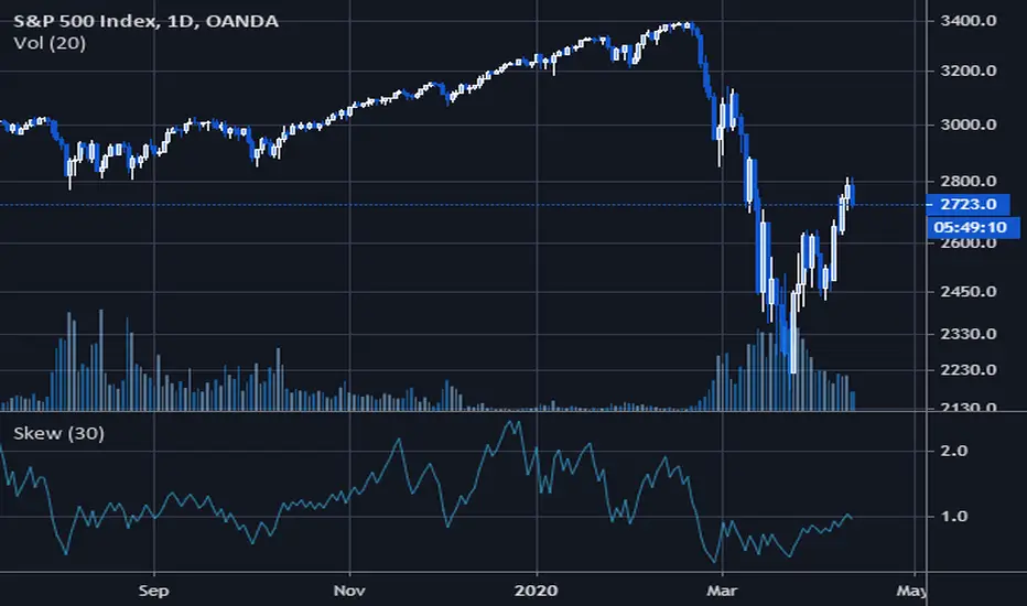
Volatility SkewThis indicator measure the historical skew of actual volatility for an individual security. It measure the volatility of up moves versus down moves over the period and gives a ratio. When the indicator is greater than one, it indicators that volatility is greater to the upside, when it is below 1 it indicates that volatility is skewed to the downside.
This is not comparable to the SKEW index, since that measures the implied volatility across option strikes, rather than using historical volatility.
Skew Index Rank-Buschi
English:
a quick and simple tampering with the SKEW Index (also known as the "Black Swan Index")
Personally, I find it quite difficult to use the SKEW Index as a reliable indicator. Nevertheless I implemented a ranking system (from 0 to 100) with the option to include a certain time period (default: 252 trading days (units)) and a moving average (default: 21 days (units)).
Feedback is most welcome to modify / improve the script.
Deutsch:
eine schnelle und einfache Bearbeitung des SKEW Index (auch als "Schwarzer Schwan Index" bekannt)
Persönlich finde ich es recht schwierig, den SKEW Index als verlässlichen Indikator zu verwenden. Trotzdem habe ich hier einfach einmal ein Ranking-System (von 0 bis 100) aufgesetzt mit der Option, einen gewissen Zeitrahmen (Standardwert: 252 Handelstage (Einheiten)) und einen gleitenden Durchschnitt (Standardwert: 21 Tage (Einheiten)) einzubinden.
Feedback ist sehr willkommen, um das Skript zu überarbeiten / zu verbessern.

Rolling Skew (Returns) - Beasley SavageSkewness is a term in statistics used to describe asymmetry from the normal distribution in a set of statistical data. Skewness can come in the form of negative skewness or positive skewness, depending on whether data points are skewed to the left and negative, or to the right and positive of the data average. A dataset that shows this characteristic differs from a normal bell curve.
