Alpha VWAP Regime🔥 Alpha VWAP Regime — Institutional VWAP Strategy (Closed Source)
Alpha VWAP Regime is a multi-layered VWAP trading system that identifies the active market regime and adapts its signals based on institutional liquidity behavior.
This strategy is closed-source because it uses a proprietary combination of VWAP structures, anchored pivot logic, band deviations, and regime detection filters that are not publicly available.
🧠 How the Strategy Works (Conceptual Explanation)
This strategy does not rely on a single VWAP line.
Instead, it builds a VWAP matrix consisting of:
1) Session VWAP
Defines fair value for the current session.
Used to detect intraday directional bias.
2) Anchored VWAP (AVWAP)
Automatically anchored to swing highs and lows (pivot-based).
Tracks where large players accumulated or distributed positions.
3) VWAP Bands (±1σ and ±2σ)
Used as dynamic volatility envelopes:
±1σ = fair-value zone / no-trade area
±2σ = mean-reversion extremes
4) Market Regime Classification (ADX-based)
The strategy determines which environment the market is in:
Trending Regime: ADX above threshold
Ranging Regime: ADX below threshold
Breakout Regime: Volume-based breakout of AVWAP
Each regime activates a different entry model.
📌 Entry Logic (High-Level Overview)
Trend Mode
Triggered only when ADX confirms a trend.
Entries occur near VWAP or −1σ using price-action confirmation.
Mean Reversion Mode
Activated when the market is ranging.
Entries target the ±2σ deviation bands.
Breakout Mode
Triggered by price crossing AVWAP with above-average volume.
Used to catch institutional continuation moves.
ALL Mode
Combines the three models for a full adaptive system.
📉 Exits & Risk Management
All stops and targets use ATR-based volatility sizing
Trend trades aim for larger targets
Mean-reversion trades aim for smaller snapback moves
Breakouts use wider stops but high R:R
🔍 How to Use the Strategy
Load the script on a clean chart
Choose your preferred regime mode (Trend / MR / Breakout / ALL)
Optionally hide VWAP indicators and display signals only
Use realistic position sizing and commissions
Evaluate performance across multiple assets and timeframes
🔒 Why It Is Closed-Source
The code uses:
A custom anchoring engine
Multi-layered regime filters
Dynamic VWAP matrix
Prop logic for bias scoring
These components were built from scratch and form a unique decision model, so the source is protected.
🇸🇦 الشرح العربي لاستراتيجية Alpha VWAP Regime
Alpha VWAP Regime هي استراتيجية تداول مؤسسية متقدمة تعتمد على تحليل السيولة، وتحديد حالة السوق (Market Regime)، ودمج عدة طبقات من VWAP داخل نموذج واحد متكيف.
الهدف من الاستراتيجية هو التداول في المناطق التي يتواجد فيها المال الذكي، وتجنب التداول في المناطق العشوائية أو منخفضة الجودة.
________________________________________
🧠 كيف تعمل الاستراتيجية؟
الاستراتيجية لا تعتمد على VWAP واحد، بل تستخدم “مصفوفة VWAP” كاملة تتكوّن من:
1) VWAP اليومي (Session VWAP)
يُستخدم لتحديد القيمة العادلة خلال الجلسة، وتحديد الاتجاه اللحظي (Intraday Bias).
________________________________________
2) VWAP المثبّت (Anchored VWAP)
يتم تثبيته تلقائيًا على:
• القمم المهمة (Swing Highs)
• القيعان المهمة (Swing Lows)
ويساعد في تحديد مناطق تمركز المؤسسات، ومناطق الانعكاس أو الاختراقات الحقيقية.
________________________________________
3) نطاقات VWAP (±1σ و ±2σ)
تُستخدم كأغلفة ديناميكية للسيولة والتقلب:
• ±1σ = منطقة القيمة العادلة (Fair-Value Zone)
→ غالبًا منطقة غير مناسبة للتداول (No-Trade Zone)
• ±2σ = مناطق التشبّع الحركي (Extremes)
→ مناسبة لاستراتيجيات الانعكاس (Mean Reversion)
________________________________________
4) تصنيف حالة السوق Market Regimes
الاستراتيجية تستخدم مؤشر ADX لتحديد حالة السوق الحالية:
حالة السوق الوصف
Trending اتجاه واضح وقوي
Ranging تذبذب بدون اتجاه
Breakout اختراق مدعوم بحجم تداول
كل Regime يفعّل نموذج دخول مختلف داخل الاستراتيجية.
________________________________________
🎯 نماذج الدخول داخل الاستراتيجية
1) نموذج الاتجاه (Trend Mode)
يعمل فقط عندما يكون السوق في اتجاه حقيقي.
يعتمد على دخول Pullbacks قرب VWAP أو نطاق −1σ مع تأكيد شموعي.
________________________________________
2) نموذج الانعكاس (Mean Reversion Mode)
يعمل فقط عندما يكون السوق متذبذبًا (Range).
الدخول عند لمس ±2σ بهدف العودة نحو VWAP.
________________________________________
3) نموذج الاختراق (Breakout Mode)
يستخدم اختراقات Anchored VWAP
ولكن بشرط وجود حجم تداول أعلى من المتوسط (Volume Confirmation).
________________________________________
4) وضع الدمج (ALL Mode)
يجمع بين النماذج الثلاثة ويجعل الاستراتيجية متكيفة تلقائيًا مع كل حالات السوق.
________________________________________
📉 الخروج وإدارة المخاطر
تستخدم الاستراتيجية نظامًا ديناميكيًا لإدارة المخاطر:
• وقف الخسارة مبني على ATR
• الأهداف مبنية على طبيعة النموذج
• الصفقات الاتجاهية تستهدف R:R أعلى
• صفقات MR أقصر وأسرع
• صفقات Breakout أوسع ولكن مدعومة بزخم قوي
________________________________________
🧩 كيفية استخدام الاستراتيجية
1. ضع الاستراتيجية على رسم بياني نظيف بدون مؤشرات إضافية
2. اختر نموذج الدخول المناسب من الإعدادات
3. فعّل أو أخفِ خطوط VWAP حسب الحاجة
4. استخدم إعدادات مخاطرة واقعية
5. اختبر الاستراتيجية على عدة أسواق وفريمات
________________________________________
🔒 سبب إغلاق الكود
تم إغلاق الكود لأنها تعتمد على:
• محرك تثبيت AVWAP خاص
• نظام Regime Detection متقدم
• مصفوفة VWAP متعددة الطبقات
• منطق دخول/خروج خاص تم تطويره بالكامل
كل ذلك يتطلب حماية الملكية الفكرية، لذا تم نشرها Closed-Source.
Phân tích Xu hướng
EMA Cross Strategy v5 (30 lots) (15 min candle only)- safe flip🚀 EMA Cross Strategy v5 (30 Lots) (15 min candle only)— Safe Flip Edition
Fully Automated | Fast | Reliable | Battle-tested
Welcome to a clean, powerful, and automation-friendly EMA crossover system.
This strategy is built for traders who want consistent trend-based entries without the risk of unwanted pyramiding or doubled positions.
🔥 How It Works
This strategy uses a fast EMA (10) crossing a slow EMA (20) to detect trend shifts:
Bullish Crossover → LONG (30 lots)
Bearish Crossover → SHORT (30 lots)
Every opposite signal safely flips the position by first closing the current trade, then opening a fresh position of exactly 30 lots.
No doubling.
No runaway position size.
No surprises.
Just clean, mechanical trend-following.
📈 Why This Strategy Stands Out
Unlike basic EMA crossbots, this version:
✔ Prevents unintended pyramiding
✔ Never over-allocates capital
✔ Works perfectly with webhook-based automation
✔ Produces stable, systematic entries
✔ Executes directional flips with precision
🔍 Backtest Highlights (1-Year)
(Backtests will vary by instrument/timeframe)
1,500+ trades executed
Profit factor above 1.27
Strong trend performance
Balanced long/short behavior
No margin calls
Consistent trade execution
This strategy thrives in trending markets and maintains strict discipline even in choppy conditions.
⚙️ Automation Ready
Designed for automated execution via webhook and API setups on supported platforms.
Just connect, run, and let the bot follow the rules without hesitation.
No emotions.
No overtrading.
No fear or greed.
Pure logic.

Golden Cross 50/200 EMATrend-following systems are characterized by having a low win rate, yet in the right circumstances (trending markets and higher timeframes) they can deliver returns that even surpass those of systems with a high win rate.
Below, I show you a simple bullish trend-following system with clear execution rules:
System Rules
-Long entries when the 50-period EMA crosses above the 200-period EMA.
-Stop Loss (SL) placed at the lowest low of the 15 candles prior to the entry candle.
-Take Profit (TP) triggered when the 50-period EMA crosses below the 200-period EMA.
Risk Management
-Initial capital: $10,000
-Position size: 10% of capital per trade
-Commissions: 0.1% per trade
Important Note:
In the code, the stop loss is defined using the swing low (15 candles), but the position size is not adjusted based on the distance to the stop loss. In other words, 10% of the equity is risked on each trade, but the actual loss on the trade is not controlled by a maximum fixed percentage of the account — it depends entirely on the stop loss level. This means the loss on a single trade could be significantly higher or lower than 10% of the account equity, depending on volatility.
Implementing leverage or reducing position size based on volatility is something I haven’t been able to include in the code, but it would dramatically improve the system’s performance. It would fix a consistent percentage loss per trade, preventing losses from fluctuating wildly with changes in volatility.
For example, we can maintain a fixed loss percentage when volatility is low by using the following formula:
Leverage = % of SL you’re willing to risk / % volatility from entry point to stop loss
And when volatility is high and would exceed the fixed percentage we want to expose per trade (if the SL is hit), we could reduce the position size accordingly.
Practical example:
Imagine we only want to risk 15% of the position value if the stop loss is triggered on Tesla (which has high volatility), but the distance to the SL represents a potential 23.57% drop. In this case, we subtract the desired risk (15%) from the actual volatility-based loss (23.57%):
23.57% − 15% = 8.57%
Now suppose we normally use $200 per trade.
To calculate 8.57% of $200:
200 × (8.57 / 100) = $17.14
Then subtract that amount from the original position size:
$200 − $17.14 = $182.86
In summary:
If we reduce the position size to $182.86 (instead of the usual $200), even if Tesla moves 23.57% against us and hits the stop loss, we would still only lose approximately 15% of the original $200 position — exactly the risk level we defined. This way, we strictly respect our risk management rules regardless of volatility swings.
I hope this clearly explains the importance of capping losses at a fixed percentage per trade. This keeps risk under control while maintaining a consistent percentage of capital invested per trade — preventing both statistical distortion of the system and the potential destruction of the account.
About the code:
Strategy declaration:
The strategy is named 'Golden Cross 50/200 EMA'.
overlay=true means it will be drawn directly on the price chart.
initial_capital=10000 sets the initial capital to $10,000.
default_qty_type=strategy.percent_of_equity and default_qty_value=10 means each trade uses 10% of available equity.
margin_long=0 indicates no margin is used for long positions (this is likely for simulation purposes only; in real trading, margin would be required).
commission_type=strategy.commission.percent and commission_value=0.1 sets a 0.1% commission per trade.
Indicators:
Calculates two EMAs: a 50-period EMA (ema50) and a 200-period EMA (ema200).
Crossover detection:
bullCross is triggered when the 50-period EMA crosses above the 200-period EMA (Golden Cross).
bearCross is triggered when the 50-period EMA crosses below the 200-period EMA (Death Cross).
Recent swing:
swingLow calculates the lowest low of the previous 15 periods.
Stop Loss:
entryStopLoss is a variable initialized as na (not available) and is updated to the current swingLow value whenever a bullCross occurs.
Entry and exit conditions:
Entry: When a bullCross occurs, the initial stop loss is set to the current swingLow and a long position is opened.
Exit on opposite signal: When a bearCross occurs, the long position is closed.
Exit on stop loss: If the price falls below entryStopLoss while a position is open, the position is closed.
Visualization:
Both EMAs are plotted (50-period in blue, 200-period in red).
Green triangles are plotted below the bar on a bullCross, and red triangles above the bar on a bearCross.
A horizontal orange line is drawn that shows the stop loss level whenever a position is open.
Alerts:
Alerts are created for:Long entry
Exit on bearish crossover (Death Cross)
Exit triggered by stop loss
Favorable Conditions:
Tesla (45-minute timeframe)
June 29, 2010 – November 17, 2025
Total net profit: $12,458.73 or +124.59%
Maximum drawdown: $1,210.40 or 8.29%
Total trades: 107
Winning trades: 27.10% (29/107)
Profit factor: 3.141
Tesla (1-hour timeframe)
June 29, 2010 – November 17, 2025
Total net profit: $7,681.83 or +76.82%
Maximum drawdown: $993.36 or 7.30%
Total trades: 75
Winning trades: 29.33% (22/75)
Profit factor: 3.157
Netflix (45-minute timeframe)
May 23, 2002 – November 17, 2025
Total net profit: $11,380.73 or +113.81%
Maximum drawdown: $699.45 or 5.98%
Total trades: 134
Winning trades: 36.57% (49/134)
Profit factor: 2.885
Netflix (1-hour timeframe)
May 23, 2002 – November 17, 2025
Total net profit: $11,689.05 or +116.89%
Maximum drawdown: $844.55 or 7.24%
Total trades: 107
Winning trades: 37.38% (40/107)
Profit factor: 2.915
Netflix (2-hour timeframe)
May 23, 2002 – November 17, 2025
Total net profit: $12,807.71 or +128.10%
Maximum drawdown: $866.52 or 6.03%
Total trades: 56
Winning trades: 41.07% (23/56)
Profit factor: 3.891
Meta (45-minute timeframe)
May 18, 2012 – November 17, 2025
Total net profit: $2,370.02 or +23.70%
Maximum drawdown: $365.27 or 3.50%
Total trades: 83
Winning trades: 31.33% (26/83)
Profit factor: 2.419
Apple (45-minute timeframe)
January 3, 2000 – November 17, 2025
Total net profit: $8,232.55 or +80.59%
Maximum drawdown: $581.11 or 3.16%
Total trades: 140
Winning trades: 34.29% (48/140)
Profit factor: 3.009
Apple (1-hour timeframe)
January 3, 2000 – November 17, 2025
Total net profit: $9,685.89 or +94.93%
Maximum drawdown: $374.69 or 2.26%
Total trades: 118
Winning trades: 35.59% (42/118)
Profit factor: 3.463
Apple (2-hour timeframe)
January 3, 2000 – November 17, 2025
Total net profit: $8,001.28 or +77.99%
Maximum drawdown: $755.84 or 7.56%
Total trades: 67
Winning trades: 41.79% (28/67)
Profit factor: 3.825
NVDA (15-minute timeframe)
January 3, 2000 – November 17, 2025
Total net profit: $11,828.56 or +118.29%
Maximum drawdown: $1,275.43 or 8.06%
Total trades: 466
Winning trades: 28.11% (131/466)
Profit factor: 2.033
NVDA (30-minute timeframe)
January 3, 2000 – November 17, 2025
Total net profit: $12,203.21 or +122.03%
Maximum drawdown: $1,661.86 or 10.35%
Total trades: 245
Winning trades: 28.98% (71/245)
Profit factor: 2.291
NVDA (45-minute timeframe)
January 3, 2000 – November 17, 2025
Total net profit: $16,793.48 or +167.93%
Maximum drawdown: $1,458.81 or 8.40%
Total trades: 172
Winning trades: 33.14% (57/172)
Profit factor: 2.927


ATR Trend + RSI Pullback Strategy [Profit-Focused]This strategy is designed to catch high-probability pullbacks during strong trends using a combination of ATR-based volatility filters, RSI exhaustion levels, and a trend-following entry model.
Strategy Logic
Rather than relying on lagging crossovers, this model waits for RSI to dip into oversold zones (below 40) while price remains above a long-term EMA (default: 200). This setup captures pullbacks in strong uptrends, allowing traders to enter early in a move while controlling risk dynamically.
To avoid entries during low-volatility conditions or sideways price action, it applies a minimum ATR filter. The ATR also defines both the stop-loss and take-profit levels, allowing the model to adapt to changing market conditions.
Exit logic includes:
A take-profit at 3× the ATR distance
A stop-loss at 1.5× the ATR distance
An optional early exit if RSI crosses above 70, signaling overbought conditions
Technical Details
Trend Filter: 200 EMA – must be rising and price must be above it
Entry Signal: RSI dips below 40 during an uptrend
Volatility Filter: ATR must be above a user-defined minimum threshold
Stop-Loss: 1.5× ATR below entry price
Take-Profit: 3.0× ATR above entry price
Exit on Overbought: RSI > 70 (optional early exit)
Backtest Settings
Initial Capital: $10,000
Position Sizing: 5% of equity per trade
Slippage: 1 tick
Commission: 0.075% per trade
Trade Direction: Long only
Timeframes Tested: 15m, 1H, and 30m on trending assets like BTCUSD, NAS100, ETHUSD
This model is tuned for positive P&L across trending environments and volatile markets.
Educational Use Only
This strategy is for educational purposes only and should not be considered financial advice. Past performance does not guarantee future results. Always validate performance on multiple markets and timeframes before using it in live trading.

Bitcoin & Ethereum Profitable Crypto Investor – FREE EditionBitcoin & Ethereum Profitable Crypto Investor – FREE Edition
by RustyTradingScripts
This is the free, simplified edition of my long-term crypto trend-following strategy designed for Bitcoin, Ethereum, and other major assets. It provides an accessible introduction to the core concepts behind the full version while remaining easy to use, transparent, and beginner-friendly.
This FREE edition focuses on a single technical component: a 102-period Simple Moving Average trend model. When price moves above the SMA, the script considers it a potential long trend environment. When the slope begins to turn down, the strategy exits the position. This creates a straightforward, rules-based framework for identifying trend shifts without emotional or discretionary decision-making.
The goal of this simplified version is to help users understand how a structured trend approach behaves during different market conditions. It demonstrates how using a slow, objective indicator can reduce noise and provide clearer long-term directional context on higher timeframes such as the 10-hour BTC chart shown in the backtest example.
What This FREE Version Includes
- Trend-based entries using a 102-period SMA
- Automatic exits when the SMA slope turns down
- Clean visual plot of the moving average
- No repainting — signals are based on confirmed bar data
- Works on BTC, ETH, and other major crypto assets
- User-adjustable SMA length for customization
What’s Not Included in This Version:
This edition intentionally focuses on the essential trend logic only.
It does NOT include the following components found in the full investor strategy:
- Linear regression smoothing
- Seasonal filters
- Price-extension filtering
- Volume-based protection
- Partial stop-loss and partial take-profit systems
- Cooldown logic after profitable trades
- RSI-based extended exits
- Multi-layered trade management modules
The purpose of this free version is to provide a clear, functional introduction to the underlying trend concept without the advanced filters and risk-management features that are part of the complete system.
How to Use It
Apply the script to your preferred asset and timeframe (commonly higher timeframes such as 4H, 8H, 10H, 12H, or 1D). The script will enter long positions when the market is trading above the SMA and exit when the slope of the average begins to point downward. Users may adjust the SMA length to match their preferred level of responsiveness.
Important Notes
This script is for educational and analytical purposes.
Historical results are not guarantees of future performance.
Always practice proper risk management and perform your own testing.
This script does not repaint.
This FREE version is meant as a helpful starting point for those exploring long-term crypto trend strategies. If you find it useful and wish to explore more advanced tools, feel free to reach out for additional information.

BTC EMA 5-9 Flip Strategy AutobotThis strategy is designed for fast and accurate trend-following trades on Bitcoin.
It uses a crossover between EMA 5 and EMA 9 to detect instant trend reversals and automatically flips between Long and Short positions.
How the strategy works
EMA 5 crossing above EMA 9 → Long
EMA 5 crossing below EMA 9 → Short
Automatically closes the opposite trade during a flip
Executes trades only on candle close
Prevents double entries with internal position-state logic
Fully compatible with automated trading via webhooks (Delta Exchange)
Why this strategy works
EMA 5–9 is extremely responsive for BTC’s volatility
Captures trend reversals early
Works best on 15-minute timeframe
Clean, simple logic without over-filtering reduces missed opportunities
Performs well in both uptrends and downtrends
Automation Ready
This strategy includes alert conditions and webhook-ready JSON for automated execution.
This is a fast-reacting BTC bot designed for intraday and swing crypto trend trading.

RubberBand Scalp NQ Strategy (V6 - High PF Focus)
================================================================================
RUBBERBAND SCALP NQ (V6 - HIGH PF FOCUS)
================================================================================
// STRATEGY OVERVIEW
// -----------------
// Instrument: NQ (Nasdaq 100 E-mini Futures)
// Style: Intraday mean-reversion scalping
// Core Idea: Price "stretches" away from VWAP, then "snaps back" → enter on strong reversal
// Session: 9:00 AM – 2:30 PM CST (America/Chicago)
// Timeframe: 1–5 min (ideal: 2–3 min)
// Position: 2 contracts, pyramiding = 0
// Commission: $2.00 per contract
// Goal: High Profit Factor via asymmetric exits (1R fixed + unlimited runner)
// KEY FILTERS
// -----------
// • Only trade when ATR(15) > 5.0 points (~$100 range) → avoids chop
// • Must be in session → forces flat at 2:30 PM
// • VWAP proximity: price must touch within 0.5 × ATR of VWAP
// ENTRY LOGIC (LONG)
// -----------------
// 1. In session & no position
// 2. Close > Open (bullish bar)
// 3. Close > highest high of last 4 bars → momentum confirmation
// 4. Close > VWAP
// 5. Low < VWAP + (0.5 × ATR) → pullback reached VWAP zone
// 6. ATR > 5.0
// 7. Bar confirmed
// → Plot green triangle below bar
// ENTRY LOGIC (SHORT) – Symmetric
// -----------------
// 1. Close < Open
// 2. Close < lowest low of last 4 bars
// 3. Close < VWAP
// 4. High > VWAP - (0.5 × ATR)
// 5. ATR > 5.0
// → Plot red triangle above bar
// STOP LOSS – DUAL SYSTEM (Widest Stop Wins)
// -----------------------------------------
// VWAP Stop (Long): VWAP - 0.20
// ATR Stop (Long): Close - min(ATR × 1.0, 15.0)
// Final Stop: MAX(VWAP Stop, ATR Stop) → then CAP at Close - 0.20
// Short: MIN of both → FLOOR at Close + 0.20
// → Max buffer: 0.20 pts = $20 (4 ticks)
// → Risk = |Entry – Final Stop|
// PROFIT TAKING – 2 CONTRACTS
// ---------------------------
// Contract #1: Fixed 1R → limit = entry + risk (long) / entry - risk (short)
// Contract #2: Trailing stop only → trail_points = risk, trail_offset = 0
// NO FIXED TAKE PROFIT ON RUNNER → lets 3R, 5R, 10R+ winners run
// BUG: Short runner uses trail_offset = 1.5 → CHANGE TO 0
// V6 IMPROVEMENTS
// ---------------
// 1. ATR_STOP_MULTIPLIER reduced from 1.5 → 1.0 → tighter average loss
// 2. Removed fixed 2R cap on runner → unlimited upside
// 3. Widest-stop logic → prevents premature stop-outs
// TRADE EXAMPLE (LONG)
// -------------------
// Entry: 18,125 (2 contracts)
// Stop: 18,110 → Risk = $300/contract
// 1R: 18,155 → Contract #1 exits (+$600)
// Runner trails by $300 → exits at 18,425 (+$6,000)
// Total P&L: +$6,600
// PERFORMANCE EXPECTATIONS
// ------------------------
// Win Rate: 40–50%
// Avg Winner: >3× avg loser
// Profit Factor: 2.0–3.5+
// Max Drawdown: <5% (with risk controls)
// DAILY CHECKLIST
// ---------------
// 2–3 min NQ chart
// Timezone: America/Chicago
// ATR > 5.0
// Price touched VWAP zone
// 4-bar breakout confirmed
// trail_offset = 0 (both sides)
// Alerts on
// Log R-multiple
// FINAL NOTES
// -----------
// This is a PROFIT FACTOR system — not a high win-rate system.
// Success = discipline + volatility + clean execution.
================================================================================

SP500 Session Gap Fade StrategySummary in one paragraph
SPX Session Gap Fade is an intraday gap fade strategy for index futures, designed around regular cash sessions on five minute charts. It helps you participate only when there is a full overnight or pre session gap and a valid intraday session window, instead of trading every open. The original part is the gap distance engine which anchors both stop and optional target to the previous session reference close at a configurable flat time, so every trade’s risk scales with the actual gap size rather than a fixed tick stop.
Scope and intent
• Markets. Primarily index futures such as ES, NQ, YM, and liquid index CFDs that exhibit overnight gaps and regular cash hours.
• Timeframes. Intraday timeframes from one minute to fifteen minutes. Default usage is five minute bars.
• Default demo used in the publication. Symbol CME:ES1! on a five minute chart.
• Purpose. Provide a simple, transparent way to trade opening gaps with a session anchored risk model and forced flat exit so you are not holding into the last part of the session.
• Limits. This is a strategy. Orders are simulated on standard candles only.
Originality and usefulness
• Unique concept or fusion. The core novelty is the combination of a strict “full gap” entry condition with a session anchored reference close and a gap distance based TP and SL engine. The stop and optional target are symmetric multiples of the actual gap distance from the previous session’s flat close, rather than fixed ticks.
• Failure mode it addresses. Fixed sized stops do not scale when gaps are unusually small or unusually large, which can either under risk or over risk the account. The session flat logic also reduces the chance of holding residual positions into late session liquidity and news.
• Testability. All key pieces are explicit in the Inputs: session window, minutes before session end, whether to use gap exits, whether TP or SL are active, and whether to allow candle based closes and forced flat. You can toggle each component and see how it changes entries and exits.
• Portable yardstick. The main unit is the absolute price gap between the entry bar open and the previous session reference close. tp_mult and sl_mult are multiples of that gap, which makes the risk model portable across contracts and volatility regimes.
Method overview in plain language
The strategy first defines a trading session using exchange time, for example 08:30 to 15:30 for ES day hours. It also defines a “flat” time a fixed number of minutes before session end. At the flat bar, any open position is closed and the bar’s close price is stored as the reference close for the next session. Inside the session, the strategy looks for a full gap bar relative to the prior bar: a gap down where today’s high is below yesterday’s low, or a gap up where today’s low is above yesterday’s high. A full gap down generates a long entry; a full gap up generates a short entry. If the gap risk engine is enabled and a valid reference close exists, the strategy measures the distance between the entry bar open and that reference close. It then sets a stop and optional target as configurable multiples of that gap distance and manages them with strategy.exit. Additional exits can be triggered by a candle color flip or by the forced flat time.
Base measures
• Range basis. The main unit is the absolute difference between the current entry bar open and the stored reference close from the previous session flat bar. That value is used as a “gap unit” and scaled by tp_mult and sl_mult to build the target and stop.
Components
• Component one: Gap Direction. Detects full gap up or full gap down by comparing the current high and low to the previous bar’s high and low. Gap down signals a long fade, gap up signals a short fade. There is no smoothing; it is a strict structural condition.
• Component two: Session Window. Only allows entries when the current time is within the configured session window. It also defines a flat time before the session end where positions are forced flat and the reference close is updated.
• Component three: Gap Distance Risk Engine. Computes the absolute distance between the entry open and the stored reference close. The stop and optional target are placed as entry ± gap_distance × multiplier so that risk scales with gap size.
• Optional component: Candle Exit. If enabled, a bullish bar closes short positions and a bearish bar closes long positions, which can shorten holding time when price reverses quickly inside the session.
• Session windows. Session logic uses the exchange time of the chart symbol. When changing symbols or venues, verify that the session time string still matches the new instrument’s cash hours.
Fusion rule
All gates are hard conditions rather than weighted scores. A trade can only open if the session window is active and the full gap condition is true. The gap distance engine only activates if a valid reference close exists and use_gap_risk is on. TP and SL are controlled by separate booleans so you can use SL only, TP only, or both. Long and short are symmetric by construction: long trades fade full gap downs, short trades fade full gap ups with mirrored TP and SL logic.
Signal rule
• Long entry. Inside the active session, when the current bar shows a full gap down relative to the previous bar (current high below prior low), the strategy opens a long position. If the gap risk engine is active, it places a gap based stop below the entry and an optional target above it.
• Short entry. Inside the active session, when the current bar shows a full gap up relative to the previous bar (current low above prior high), the strategy opens a short position. If the gap risk engine is active, it places a gap based stop above the entry and an optional target below it.
• Forced flat. At the configured flat time before session end, any open position is closed and the close price of that bar becomes the new reference close for the following session.
• Candle based exit. If enabled, a bearish bar closes longs, and a bullish bar closes shorts, regardless of where TP or SL sit, as long as a position is open.
What you will see on the chart
• Markers on entry bars. Standard strategy entry markers labeled “long” and “short” on the gap bars where trades open.
• Exit markers. Standard exit markers on bars where either the gap stop or target are hit, or where a candle exit or forced flat close occurs. Exit IDs “long_gap” and “short_gap” label gap based exits.
• Reference levels. Horizontal lines for the current long TP, long SL, short TP, and short SL while a position is open and the gap engine is enabled. They update when a new trade opens and disappear when flat.
• Session background. This version does not add background shading for the session; session logic runs internally based on time.
• No on chart table. All decisions are visible through orders and exit levels. Use the Strategy Tester for performance metrics.
Inputs with guidance
Session Settings
• Trading session (sess). Session window in exchange time. Typical value uses the regular cash session for each contract, for example “0830-1530” for ES. Adjust if your broker or symbol uses different hours.
• Minutes before session end to force exit (flat_before_min). Minutes before the session end where positions are forced flat and the reference close is stored. Typical range is 15 to 120. Raising it closes trades earlier in the day; lowering it allows trades later in the session.
Gap Risk
• Enable gap based TP/SL (use_gap_risk). Master switch for the gap distance exit engine. Turning it off keeps entries and forced flat logic but removes automatic TP and SL placement.
• Use TP limit from gap (use_gap_tp). Enables gap based profit targets. Typical values are true for structured exits or false if you want to manage exits manually and only keep a stop.
• Use SL stop from gap (use_gap_sl). Enables gap based stop losses. This should normally remain true so that each trade has a defined initial risk in ticks.
• TP multiplier of gap distance (tp_mult). Multiplier applied to the gap distance for the target. Typical range is 0.5 to 2.0. Raising it places the target further away and reduces hit frequency.
• SL multiplier of gap distance (sl_mult). Multiplier applied to the gap distance for the stop. Typical range is 0.5 to 2.0. Raising it widens the stop and increases risk per trade; lowering it tightens the stop and may increase the number of small losses.
Exit Controls
• Exit with candle logic (use_candle_exit). If true, closes shorts on bullish candles and longs on bearish candles. Useful when you want to react to intraday reversal bars even if TP or SL have not been reached.
• Force flat before session end (use_forced_flat). If true, guarantees you are flat by the configured flat time and updates the reference close. Turn this off only if you understand the impact on overnight risk.
Filters
There is no separate trend or volatility filter in this version. All trades depend on the presence of a full gap bar inside the session. If you need extra filtering such as ATR, volume, or higher timeframe bias, they should be added explicitly and documented in your own fork.
Usage recipes
Intraday conservative gap fade
• Timeframe. Five minute chart on ES regular session.
• Gap risk. use_gap_risk = true, use_gap_tp = true, use_gap_sl = true.
• Multipliers. tp_mult around 0.7 to 1.0 and sl_mult around 1.0.
• Exits. use_candle_exit = false, use_forced_flat = true. Focus on the structured TP and SL around the gap.
Intraday aggressive gap fade
• Timeframe. Five minute chart.
• Gap risk. use_gap_risk = true, use_gap_tp = false, use_gap_sl = true.
• Multipliers. sl_mult around 0.7 to 1.0.
• Exits. use_candle_exit = true, use_forced_flat = true. Entries fade full gaps, stops are tight, and candle color flips flatten trades early.
Higher timeframe gap tests
• Timeframe. Fifteen minute or sixty minute charts on instruments with regular gaps.
• Gap risk. Keep use_gap_risk = true. Consider slightly higher sl_mult if gaps are structurally wider on the higher timeframe.
• Note. Expect fewer trades and be careful with sample size; multi year data is recommended.
Properties visible in this publication
• On average our risk for each position over the last 200 trades is 0.4% with a max intraday loss of 1.5% of the total equity in this case of 100k $ with 1 contract ES. For other assets, recalculations and customizations has to be applied.
• Initial capital. 100 000.
• Base currency. USD.
• Default order size method. Fixed with size 1 contract.
• Pyramiding. 0.
• Commission. Flat 2 USD per order in the Strategy Tester Properties. (2$ buying + 2$selling)
• Slippage. One tick in the Strategy Tester Properties.
• Process orders on close. ON.
Realism and responsible publication
• No performance claims are made. Past results do not guarantee future outcomes.
• Costs use a realistic flat commission and one tick of slippage per trade for ES class futures.
• Default sizing with one contract on a 100 000 reference account targets modest per trade risk. In practice, extreme slippage or gap through events can exceed this, so treat the one and a half percent risk target as a design goal, not a guarantee.
• All orders are simulated on standard candles. Shapes can move while a bar is forming and settle on bar close.
Honest limitations and failure modes
• Economic releases, thin liquidity, and limit conditions can break the assumptions behind the simple gap model and lead to slippage or skipped fills.
• Symbols with very frequent or very large gaps may require adjusted multipliers or alternative risk handling, especially in high volatility regimes.
• Very quiet periods without clean gaps will produce few or no trades. This is expected behavior, not a bug.
• Session windows follow the exchange time of the chart. Always confirm that the configured session matches the symbol.
• When both the stop and target lie inside the same bar’s range, the TradingView engine decides which is hit first based on its internal intrabar assumptions. Without bar magnifier, tie handling is approximate.
Legal
Education and research only. This strategy is not investment advice. You remain responsible for all trading decisions. Always test on historical data and in simulation with realistic costs before considering any live use.

MSB Trend Breakout Strategy V7**MSB Trend Breakout Strategy V7**
This is the full, high-precision automated strategy designed for disciplined traders who understand directional price action. The script functions as a robust **entry and trade management tool** following two proprietary concepts:
**1. Trend Confirmation:** A customized Moving Average filter is utilized to ensure entries strictly align with the dominant market flow.
**2. Momentum Confirmation:** The system uses a specific short-term **multi-bar breakout range** to pinpoint high-probability entries at the start of a momentum shift, avoiding choppy market conditions.
**Key Features:**
* **Automated Risk Management:** Includes complete dynamic Stop Loss (SL) and Take Profit (TP) order management to ensure capital preservation.
* **Time Filter:** Optimizes performance by filtering signals to the most liquid Forex trading hours (01:00 to 19:00, broker time).
**PREREQUISITE FOR ACCESS:**
This is an advanced tool. To utilize the strategy effectively, the user should have a foundational understanding of directional bias and trade management principles.
---
**Important Note & Risk Disclosure:**
This strategy is published under **Invite-only** protection. The script does not provide financial advice or guarantee profits. Past performance is not indicative of future results.

Moving Average Band StrategyOverview
The Moving Average Band Strategy is a fully customizable breakout and trend-continuation system designed for traders who need both simplicity and control.
The strategy creates adaptive bands around a user-selected moving average and executes trades when price breaks out of these bands, with advanced risk-management settings including optional Risk:Reward targets.
This script is suitable for intraday, swing, and positional traders across all markets — equities, futures, crypto, and forex.
Key Features
✔ Six Moving Average Types
Choose the MA that best matches your trading style:
SMA
EMA
WMA
HMA
VWMA
RMA
✔ Dynamic Bands
Upper Band built from MA of highs
Lower Band built from MA of lows
Adjustable band offset (%)
Color-coded band fill indicating price position
✔ Configurable Strategy Preferences
Toggle Long and/or Short trades
Toggle Risk:Reward Take-Profit
Adjustable Risk:Reward Ratio
Default position sizing: % of equity (configurable via strategy settings)
Entry Conditions
Long Entry
A long trade triggers when:
Price crosses above the Upper Band
Long trades are enabled
No existing long position is active
Short Entry
A short trade triggers when:
Price crosses below the Lower Band
Short trades are enabled
No existing short position is active
Clear entry markers and price labels appear on the chart.
Risk Management
This strategy includes a complete set of risk-controls:
Stop-Loss (Fixed at Entry)
Long SL: Lower Band
Short SL: Upper Band
These levels remain constant for the entire trade.
Optional Risk:Reward Take-Profit
Enabled/disabled using a toggle switch.
When enabled:
Long TP = Entry + (Risk × Risk:Reward Ratio)
Short TP = Entry – (Risk × Risk:Reward Ratio)
When disabled:
Exits are handled by reverse crossover signals.
Exit Conditions
Long Exit
Stop-Loss Hit (touch-based)
Take-Profit Hit (if enabled)
Reverse Band Crossover (if TP disabled)
Short Exit
Stop-Loss Hit (touch-based)
Take-Profit Hit (if enabled)
Reverse Band Crossover (if TP disabled)
Exit markers and price labels are plotted automatically.
Visual Tools
To improve clarity:
Upper & Lower Band (blue, adjustable width)
Middle Line
Dynamic band fill (green/red/yellow)
SL & TP line plotting when in position
Entry/Exit markers
Price labels for all executed trades
These are built to help users visually follow the strategy logic.
Alerts Included
Every trading event is covered:
Long Entry
Short Entry
Long SL / TP / Cross Exit
Short SL / TP / Cross Exit
Combined Alert for webhook/automation (JSON-formatted)
Perfect for algo trading, Discord bots, or automation platforms.
Best For
This strategy performs best in:
Trending markets
Breakout environments
High-momentum instruments
Clean intraday swings
Works seamlessly on:
Stocks
Index futures
Commodities
Crypto
Forex
⚠️ Important Disclaimer
This script is for educational purposes only.
Trading involves risk. Backtest results are not indicative of future performance.
Always validate settings and use proper position sizing.

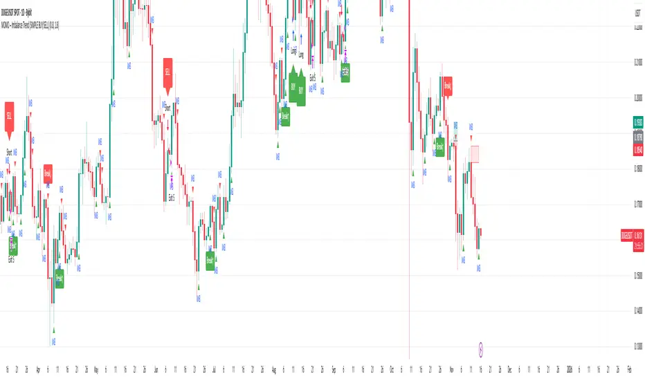
MOMO – Imbalance Trend (SIMPLE BUY/SELL)MOMO – Imbalance Trend (SIMPLE BUY/SELL)
This strategy combines trend breaks, imbalance detection, and first-tap supply/demand entries to create a clean and disciplined trading model.
It automatically highlights imbalance candles, draws fresh zones, and waits for the first retest to deliver precise BUY and SELL signals.
Performance
On optimized settings, this strategy shows an estimated 57%–70% win-rate, depending on the asset and timeframe.
Actual performance may vary, but the model is built for consistency, discipline, and improved decision-making.
How it works
Detects trend structure shifts (BOS / Break of Trend)
Identifies displacement (imbalance) candles
Creates supply and demand zones from imbalance origin
Waits for first tap only (no second chances)
Confirms direction using trend logic
Generates clean BUY/SELL arrows
Automatic SL/TP based on user settings
Features
Clean BUY/SELL markers
Auto-drawn supply & demand zones
Trend break markers
Imbalance tags
Smart first-tap confirmation
Customizable stop loss & take profit
Works on crypto, gold, forex, indices
Best on M5–H1 for day trading
Note
This strategy is designed for day traders who want clarity, structure, and zero emotional trading.
Use it with discipline — and it will serve you well.
Good luck, soldier.
Fractional Candlestick Long Only Experimental V10Fractional Candlestick Long-Only Strategy – Technical Description
This document provides a professional English description of the "Fractional Candlestick Long Only Experimental V6" strategy using pure CF/AB fractional kernels and wavelet-based filtering.
1. Fractional Candlesticks (CF / AB)
The strategy computes two fractional representations of price using Caputo–Fabrizio (CF) and Atangana–Baleanu (AB) kernels. These provide long-memory filtering without EMA approximations. Both CF and AB versions are applied to O/H/L/C, producing fractional candlesticks and fractional Heikin-Ashi variants.
2. Trend Stack Logic
Trend confirmation is based on a 4-component stack:
- CF close > AB close
- HA_CF close > HA_AB close
- HA_CF bullish
- HA_AB bullish
The user selects how many components must align (4, 3, or any 2).
3. Wavelet Filtering
A wavelet transform (Haar, Daubechies-4, Mexican Hat) is applied to a chosen source (e.g., HA_CF close). The wavelet response is used as:
- entry filter (4 modes)
- exit filter (4 modes)
Wavelet modes: off, confirm, wavelet-only, block adverse signals.
4. Trailing System
Trailing stop uses fractional AB low × buffer, providing long-memory dynamic trailing behavior. A fractional trend channel (CF/AB lows vs HA highs) is also plotted.
5. Exit Framework
Exit options include: stack flip, CF

Supertrend +QQE + DEMASupertrend + QQE + DEMA — Strategy
Inspired by UNITED and my best friend ChatGPT
This strategy combines dual Supertrends, a QQE trend filter, and a 200-period DEMA directional filter to generate structured, trend-aligned entries. It is designed for Heikin Ashi charts , where trend noise is reduced and swing structure becomes clearer.
How It Works
The system fires a trade only when all conditions agree:
1. Both Supertrends flip in the same direction
This identifies strong directional shifts and removes weak reversals.
2. QQE Trend Confirmation
QQE acts as a momentum filter, requiring either a green (bullish) or red (bearish) state with optional consecutive-bar confirmation.
3. 200 DEMA Filter
Only longs above the DEMA and only shorts below the DEMA.
This keeps trades aligned with the higher-timeframe trend.
Because each component filters the other, signals are high-quality, controlled, and structured rather than frequent or reactive.
Expected Performance
Based on the design and typical market testing, this combination yields a 50–70% win rate, depending on:
The market (best on indices like NQ/MNQ, ES/MES, DAX, etc.)
Volatility conditions
Whether used on Heikin Ashi , which increases trend-cleanliness and reduces chop
Timeframe (1m–5m often optimal for intraday)
The system avoids rapid flip-flopping by using “arm → confirm → fire once” logic, which further improves win consistency and reduces whipsaw losses.
How to Properly Use It (IMPORTANT)
This strategy is meant to be run on a Heikin Ashi chart.
Why?
Heikin Ashi smooths candles, giving clearer:
Trend transitions
Pullbacks
Momentum continuation
Supertrend reliability
Running this on normal candles will still work, but the win rate and smoothness drop significantly because Supertrend + QQE respond more cleanly to HA structure.
Trade Behavior
Longs trigger when both Supertrends flip up, QQE is bullish, and price is above DEMA.
Shorts trigger when both Supertrends flip down, QQE is bearish, and price is below DEMA.
Strategy closes when the opposite Supertrend flip occurs.
Alerts fire automatically for buy/sell confirmations.
Best Use Cases
Intraday trend trading
Momentum continuation after a confirmed reversal
Avoiding chop with multi-layer confirmation
Backtesting rule-based execution

Reversal Point Dynamics - Machine Learning⇋ Reversal Point Dynamics - Machine Learning
RPD Machine Learning: Self-Adaptive Multi-Armed Bandit Trading System
RPD Machine Learning is an advanced algorithmic trading system that implements genuine machine learning through contextual multi-armed bandits, reinforcement learning, and online adaptation. Unlike traditional indicators that use fixed rules, RPD learns from every trade outcome , automatically discovers which strategies work in current market conditions, and continuously adapts without manual intervention .
Core Innovation: The system deploys six distinct trading policies (ranging from aggressive trend-following to conservative range-bound strategies) and uses LinUCB contextual bandit algorithms with Random Fourier Features to learn which policy performs best in each market regime. After the initial learning phase (50-100 trades), the system achieves autonomous adaptation , automatically shifting between policies as market conditions evolve.
Target Users: Quantitative traders, algorithmic trading developers, systematic traders, and data-driven investors who want a system that adapts over time . Suitable for stocks, futures, forex, and cryptocurrency on any liquid instrument with >100k daily volume.
The Problem This System Solves
Traditional Technical Analysis Limitations
Most trading systems suffer from three fundamental challenges :
Fixed Parameters: Static settings (like "buy when RSI < 30") work well in backtests but may struggle when markets change character. What worked in low-volatility environments may not work in high-volatility regimes.
Strategy Degradation: Manual optimization (curve-fitting) produces systems that perform well on historical data but may underperform in live trading. The system never adapts to new market conditions.
Cognitive Overload: Running multiple strategies simultaneously forces traders to manually decide which one to trust. This leads to hesitation, late entries, and inconsistent execution.
How RPD Machine Learning Addresses These Challenges
Automated Strategy Selection: Instead of requiring you to choose between trend-following and mean-reversion strategies, RPD runs all six policies simultaneously and uses machine learning to automatically select the best one for current conditions. The decision happens algorithmically, removing human hesitation.
Continuous Learning: After every trade, the system updates its understanding of which policies are working. If the market shifts from trending to ranging, RPD automatically detects this through changing performance patterns and adjusts selection accordingly.
Context-Aware Decisions: Unlike simple voting systems that treat all conditions equally, RPD analyzes market context (ADX regime, entropy levels, volatility state, volume patterns, time of day, historical performance) and learns which combinations of context features correlate with policy success.
Machine Learning Architecture: What Makes This "Real" ML
Component 1: Contextual Multi-Armed Bandits (LinUCB)
What Is a Multi-Armed Bandit Problem?
Imagine facing six slot machines, each with unknown payout rates. The exploration-exploitation dilemma asks: Should you keep pulling the machine that's worked well (exploitation) or try others that might be better (exploration)? RPD solves this for trading policies.
Academic Foundation:
RPD implements Linear Upper Confidence Bound (LinUCB) from the research paper "A Contextual-Bandit Approach to Personalized News Article Recommendation" (Li et al., 2010, WWW Conference). This algorithm is used in content recommendation and ad placement systems.
How It Works:
Each policy (AggressiveTrend, ConservativeRange, VolatilityBreakout, etc.) is treated as an "arm." The system maintains:
Reward History: Tracks wins/losses for each policy
Contextual Features: Current market state (8-10 features including ADX, entropy, volatility, volume)
Uncertainty Estimates: Confidence in each policy's performance
UCB Formula: predicted_reward + α × uncertainty
The system selects the policy with highest UCB score , balancing proven performance (predicted_reward) with potential for discovery (uncertainty bonus). Initially, all policies have high uncertainty, so the system explores broadly. After 50-100 trades, uncertainty decreases, and the system focuses on known-performing policies.
Why This Matters:
Traditional systems pick strategies based on historical backtests or user preference. RPD learns from actual outcomes in your specific market, on your timeframe, with your execution characteristics.
Component 2: Random Fourier Features (RFF)
The Non-Linearity Challenge:
Market relationships are often non-linear. High ADX may indicate favorable conditions when volatility is normal, but unfavorable when volatility spikes. Simple linear models struggle to capture these interactions.
Academic Foundation:
RPD implements Random Fourier Features from "Random Features for Large-Scale Kernel Machines" (Rahimi & Recht, 2007, NIPS). This technique approximates kernel methods (like Support Vector Machines) while maintaining computational efficiency for real-time trading.
How It Works:
The system transforms base features (ADX, entropy, volatility, etc.) into a higher-dimensional space using random projections and cosine transformations:
Input: 8 base features
Projection: Through random Gaussian weights
Transformation: cos(W×features + b)
Output: 16 RFF dimensions
This allows the bandit to learn non-linear relationships between market context and policy success. For example: "AggressiveTrend performs well when ADX >25 AND entropy <0.6 AND hour >9" becomes naturally encoded in the RFF space.
Why This Matters:
Without RFF, the system could only learn "this policy has X% historical performance." With RFF, it learns "this policy performs differently in these specific contexts" - enabling more nuanced selection.
Component 3: Reinforcement Learning Stack
Beyond bandits, RPD implements a complete RL framework :
Q-Learning: Value-based RL that learns state-action values. Maps 54 discrete market states (trend×volatility×RSI×volume combinations) to 5 actions (4 policies + no-trade). Updates via Bellman equation after each trade. Converges toward optimal policy after 100-200 trades.
TD(λ) with Eligibility Traces: Extension of Q-Learning that propagates credit backwards through time . When a trade produces an outcome, TD(λ) updates not just the final state-action but all states visited during the trade, weighted by eligibility decay (λ=0.90). This accelerates learning from multi-bar trades.
Policy Gradient (REINFORCE): Learns a stochastic policy directly from 12 continuous market features without discretization. Uses gradient ascent to increase probability of actions that led to positive outcomes. Includes baseline (average reward) for variance reduction.
Meta-Learning: The system learns how to learn by adapting its own learning rates based on feature stability and correlation with outcomes. If a feature (like volume ratio) consistently correlates with success, its learning rate increases. If unstable, rate decreases.
Why This Matters:
Q-Learning provides fast discrete decisions. Policy Gradient handles continuous features. TD(λ) accelerates learning. Meta-learning optimizes the optimization. Together, they create a robust, multi-approach learning system that adapts more quickly than any single algorithm.
Component 4: Policy Momentum Tracking (v2 Feature)
The Recency Challenge:
Standard bandits treat all historical data equally. If a policy performed well historically but struggles in current conditions due to regime shift, the system may be slow to adapt because historical success outweighs recent underperformance.
RPD's Solution:
Each policy maintains a ring buffer of the last 10 outcomes. The system calculates:
Momentum: recent_win_rate - global_win_rate (range: -1 to +1)
Confidence: consistency of recent results (1 - variance)
Policies with positive momentum (recent outperformance) get an exploration bonus. Policies with negative momentum and high confidence (consistent recent underperformance) receive a selection penalty.
Effect: When markets shift, the system detects the shift more quickly through momentum tracking, enabling faster adaptation than standard bandits.
Signal Generation: The Core Algorithm
Multi-Timeframe Fractal Detection
RPD identifies reversal points using three complementary methods :
1. Quantum State Analysis:
Divides price range into discrete states (default: 6 levels)
Peak signals require price in top states (≥ state 5)
Valley signals require price in bottom states (≤ state 1)
Prevents mid-range signals that may struggle in strong trends
2. Fractal Geometry:
Identifies swing highs/lows using configurable fractal strength
Confirms local extremum with neighboring bars
Validates reversal only if price crosses prior extreme
3. Multi-Timeframe Confirmation:
Analyzes higher timeframe (4× default) for alignment
MTF confirmation adds probability bonus
Designed to reduce false signals while preserving valid setups
Probability Scoring System
Each signal receives a dynamic probability score (40-99%) based on:
Base Components:
Trend Strength: EMA(velocity) / ATR × 30 points
Entropy Quality: (1 - entropy) × 10 points
Starting baseline: 40 points
Enhancement Bonuses:
Divergence Detection: +20 points (price/momentum divergence)
RSI Extremes: +8 points (RSI >65 for peaks, <40 for valleys)
Volume Confirmation: +5 points (volume >1.2× average)
Adaptive Momentum: +10 points (strong directional velocity)
MTF Alignment: +12 points (higher timeframe confirms)
Range Factor: (high-low)/ATR × 3 - 1.5 points (volatility adjustment)
Regime Bonus: +8 points (trending ADX >25 with directional agreement)
Penalties:
High Entropy: -5 points (entropy >0.85, chaotic price action)
Consolidation Regime: -10 points (ADX <20, no directional conviction)
Final Score: Clamped to 40-99% range, classified as ELITE (>85%), STRONG (75-85%), GOOD (65-75%), or FAIR (<65%)
Entropy-Based Quality Filter
What Is Entropy?
Entropy measures randomness in price changes . Low entropy indicates orderly, directional moves. High entropy indicates chaotic, unpredictable conditions.
Calculation:
Count up/down price changes over adaptive period
Calculate probability: p = ups / total_changes
Shannon entropy: -p×log(p) - (1-p)×log(1-p)
Normalized to 0-1 range
Application:
Entropy <0.5: Highly ordered (ELITE signals possible)
Entropy 0.5-0.75: Mixed (GOOD signals)
Entropy >0.85: Chaotic (signals blocked or heavily penalized)
Why This Matters:
Prevents trading during choppy, news-driven conditions where technical patterns may be less reliable. Automatically raises quality bar when market is unpredictable.
Regime Detection & Market Microstructure - ADX-Based Regime Classification
RPD uses Wilder's Average Directional Index to classify markets:
Bull Trend: ADX >25, +DI > -DI (directional conviction bullish)
Bear Trend: ADX >25, +DI < -DI (directional conviction bearish)
Consolidation: ADX <20 (no directional conviction)
Transitional: ADX 20-25 (forming direction, ambiguous)
Filter Logic:
Blocks all signals during Transitional regime (avoids trading during uncertain conditions)
Blocks Consolidation signals unless ADX ≥ Min Trend Strength
Adds probability bonus during strong trends (ADX >30)
Effect: Designed to reduce signal frequency while focusing on higher-quality setups.
Divergence Detection
Bearish Divergence:
Price makes higher high
Velocity (price momentum) makes lower high
Indicates weakening upward pressure → SHORT signal quality boost
Bullish Divergence:
Price makes lower low
Velocity makes higher low
Indicates weakening downward pressure → LONG signal quality boost
Bonus: Adds probability points and additional acceleration factor. Divergence signals have historically shown higher success rates in testing.
Hierarchical Policy System - The Six Trading Policies
1. AggressiveTrend (Policy 0):
Probability Threshold: 60% (trades more frequently)
Entropy Threshold: 0.70 (tolerates moderate chaos)
Stop Multiplier: 2.5× ATR (wider stops for trends)
Target Multiplier: 5.0R (larger targets)
Entry Mode: Pyramid (scales into winners)
Best For: Strong trending markets, breakouts, momentum continuation
2. ConservativeRange (Policy 1):
Probability Threshold: 75% (more selective)
Entropy Threshold: 0.60 (requires order)
Stop Multiplier: 1.8× ATR (tighter stops)
Target Multiplier: 3.0R (modest targets)
Entry Mode: Single (one-shot entries)
Best For: Range-bound markets, low volatility, mean reversion
3. VolatilityBreakout (Policy 2):
Probability Threshold: 65% (moderate)
Entropy Threshold: 0.80 (accepts high entropy)
Stop Multiplier: 3.0× ATR (wider stops)
Target Multiplier: 6.0R (larger targets)
Entry Mode: Tiered (splits entry)
Best For: Compression breakouts, post-consolidation moves, gap opens
4. EntropyScalp (Policy 3):
Probability Threshold: 80% (very selective)
Entropy Threshold: 0.40 (requires extreme order)
Stop Multiplier: 1.5× ATR (tightest stops)
Target Multiplier: 2.5R (quick targets)
Entry Mode: Single
Best For: Low-volatility grinding moves, tight ranges, highly predictable patterns
5. DivergenceHunter (Policy 4):
Probability Threshold: 70% (quality-focused)
Entropy Threshold: 0.65 (balanced)
Stop Multiplier: 2.2× ATR (moderate stops)
Target Multiplier: 4.5R (balanced targets)
Entry Mode: Tiered
Best For: Divergence-confirmed reversals, exhaustion moves, trend climax
6. AdaptiveBlend (Policy 5):
Probability Threshold: 68% (balanced)
Entropy Threshold: 0.75 (balanced)
Stop Multiplier: 2.0× ATR (standard)
Target Multiplier: 4.0R (standard)
Entry Mode: Single
Best For: Mixed conditions, general trading, fallback when no clear regime
Policy Clustering (Advanced/Extreme Modes)
Policies are grouped into three clusters based on regime affinity:
Cluster 1 (Trending): AggressiveTrend, DivergenceHunter
High regime affinity (0.8): Performs well when ADX >25
Moderate vol affinity (0.6): Works in various volatility
Cluster 2 (Ranging): ConservativeRange, AdaptiveBlend
Low regime affinity (0.3): Better suited for ADX <20
Low vol affinity (0.4): Optimized for calm markets
Cluster 3 (Breakout): VolatilityBreakout
Moderate regime affinity (0.6): Works in multiple regimes
High vol affinity (0.9): Requires high volatility for optimal characteristics
Hierarchical Selection Process:
Calculate cluster scores based on current regime and volatility
Select best-matching cluster
Run UCB selection within chosen cluster
Apply momentum boost/penalty
This two-stage process reduces learning time - instead of choosing among 6 policies from scratch, system first narrows to 1-2 policies per cluster, then optimizes within cluster.
Risk Management & Position Sizing
Dynamic Kelly Criterion Sizing (Optional)
Traditional Fixed Sizing Challenge:
Using the same position size for all signal probabilities may be suboptimal. Higher-probability signals could justify larger positions, lower-probability signals smaller positions.
Kelly Formula:
f = (p × b - q) / b
Where:
p = win probability (from signal score)
q = loss probability (1 - p)
b = win/loss ratio (average_win / average_loss)
f = fraction of capital to risk
RPD Implementation:
Uses Fractional Kelly (1/4 Kelly default) for safety. Full Kelly is theoretically optimal but can recommend large position sizes. Fractional Kelly reduces volatility while maintaining adaptive sizing benefits.
Enhancements:
Probability Bonus: Normalize(prob, 65, 95) × 0.5 multiplier
Divergence Bonus: Additional sizing on divergence signals
Regime Bonus: Additional sizing during strong trends (ADX >30)
Momentum Adjustment: Hot policies receive sizing boost, cold policies receive reduction
Safety Rails:
Minimum: 1 contract (floor)
Maximum: User-defined cap (default 10 contracts)
Portfolio Heat: Max total risk across all positions (default 4% equity)
Multi-Mode Stop Loss System
ATR Mode (Default):
Stop = entry ± (ATR × base_mult × policy_mult)
Consistent risk sizing
Ignores market structure
Best for: Futures, forex, algorithmic trading
Structural Mode:
Finds swing low (long) or high (short) over last 20 bars
Identifies fractal pivots within lookback
Places stop below/above structure + buffer (0.1× ATR)
Best for: Stocks, instruments that respect structure
Hybrid Mode (Intelligent):
Attempts structural stop first
Falls back to ATR if:
Structural level is invalid (beyond entry)
Structural stop >2× ATR away (too wide)
Best for: Mixed instruments, adaptability
Dynamic Adjustments:
Breakeven: Move stop to entry + 1 tick after 1.0R profit
Trailing: Trail stop 0.8R behind price after 1.5R profit
Timeout: Force close after 30 bars (optional)
Tiered Entry System
Challenge: Equal sizing on all signals may not optimize capital allocation relative to signal quality.
Solution:
Tier 1 (40% of size): Enters immediately on all signals
Tier 2 (60% of size): Enters only if probability ≥ Tier 2 trigger (default 75%)
Example:
Calculated optimal size: 10 contracts
Signal probability: 72%
Tier 2 trigger: 75%
Result: Enter 4 contracts only (Tier 1)
Same signal at 80% probability
Result: Enter 10 contracts (4 Tier 1 + 6 Tier 2)
Effect: Automatically scales size to signal quality, optimizing capital allocation.
Performance Optimization & Learning Curve
Warmup Phase (First 50 Trades)
Purpose: Ensure all policies get tested before system focuses on preferred strategies.
Modifications During Warmup:
Probability thresholds reduced 20% (65% becomes 52%)
Entropy thresholds increased 20% (more permissive)
Exploration rate stays high (30%)
Confidence width (α) doubled (more exploration)
Why This Matters:
Without warmup, system might commit to early-performing policy without testing alternatives. Warmup forces thorough exploration before focusing on best-performing strategies.
Curriculum Learning
Phase 1 (Trades 1-50): Exploration
Warmup active
All policies tested
High exploration (30%)
Learning fundamental patterns
Phase 2 (Trades 50-100): Refinement
Warmup ended, thresholds normalize
Exploration decaying (30% → 15%)
Policy preferences emerging
Meta-learning optimizing
Phase 3 (Trades 100-200): Specialization
Exploration low (15% → 8%)
Clear policy preferences established
Momentum tracking fully active
System focusing on learned patterns
Phase 4 (Trades 200+): Maturity
Exploration minimal (8% → 5%)
Regime-policy relationships learned
Auto-adaptation to market shifts
Stable performance expected
Convergence Indicators
System is learning well when:
Policy switch rate decreasing over time (initially ~50%, should drop to <20%)
Exploration rate decaying smoothly (30% → 5%)
One or two policies emerge with >50% selection frequency
Performance metrics stabilizing over time
Consistent behavior in similar market conditions
System may need adjustment when:
Policy switch rate >40% after 100 trades (excessive exploration)
Exploration rate not decaying (parameter issue)
All policies showing similar selection (not differentiating)
Performance declining despite relaxed thresholds (underlying signal issue)
Highly erratic behavior after learning phase
Advanced Features
Attention Mechanism (Extreme Mode)
Challenge: Not all features are equally important. Trading hour might matter more than price-volume correlation, but standard approaches treat them equally.
Solution:
Each RFF dimension has an importance weight . After each trade:
Calculate correlation: sign(feature - 0.5) × sign(reward)
Update importance: importance += correlation × 0.01
Clamp to range
Effect: Important features get amplified in RFF transformation, less important features get suppressed. System learns which features correlate with successful outcomes.
Temporal Context (Extreme Mode)
Challenge: Current market state alone may be incomplete. Historical context (was volatility rising or falling?) provides additional information.
Solution:
Includes 3-period historical context with exponential decay (0.85):
Current features (weight 1.0)
1 bar ago (weight 0.85)
2 bars ago (weight 0.72)
Effect: Captures momentum and acceleration of market features. System learns patterns like "rising volatility with falling entropy" that may precede significant moves.
Transfer Learning via Episodic Memory
Short-Term Memory (STM):
Last 20 trades
Fast adaptation to immediate regime
High learning rate
Long-Term Memory (LTM):
Condensed historical patterns
Preserved knowledge from past regimes
Low learning rate
Transfer Mechanism:
When STM fills (20 trades), patterns consolidated into LTM . When similar regime recurs later, LTM provides faster adaptation than starting from scratch.
Practical Implementation Guide - Recommended Settings by Instrument
Futures (ES, NQ, CL):
Adaptive Period: 20-25
ML Mode: Advanced
RFF Dimensions: 16
Policies: 6
Base Risk: 1.5%
Stop Mode: ATR or Hybrid
Timeframe: 5-15 min
Forex Majors (EURUSD, GBPUSD):
Adaptive Period: 25-30
ML Mode: Advanced
RFF Dimensions: 16
Policies: 6
Base Risk: 1.0-1.5%
Stop Mode: ATR
Timeframe: 5-30 min
Cryptocurrency (BTC, ETH):
Adaptive Period: 20-25
ML Mode: Extreme (handles non-stationarity)
RFF Dimensions: 32 (captures complexity)
Policies: 6
Base Risk: 1.0% (volatility consideration)
Stop Mode: Hybrid
Timeframe: 15 min - 4 hr
Stocks (Large Cap):
Adaptive Period: 25-30
ML Mode: Advanced
RFF Dimensions: 16
Policies: 5-6
Base Risk: 1.5-2.0%
Stop Mode: Structural or Hybrid
Timeframe: 15 min - Daily
Scaling Strategy
Phase 1 (Testing - First 50 Trades):
Max Contracts: 1-2
Goal: Validate system on your instrument
Monitor: Performance stabilization, learning progress
Phase 2 (Validation - Trades 50-100):
Max Contracts: 2-3
Goal: Confirm learning convergence
Monitor: Policy stability, exploration decay
Phase 3 (Scaling - Trades 100-200):
Max Contracts: 3-5
Enable: Kelly sizing (1/4 Kelly)
Goal: Optimize capital efficiency
Monitor: Risk-adjusted returns
Phase 4 (Full Deployment - Trades 200+):
Max Contracts: 5-10
Enable: Full momentum tracking
Goal: Sustained consistent performance
Monitor: Ongoing adaptation quality
Limitations & Disclaimers
Statistical Limitations
Learning Sample Size: System requires minimum 50-100 trades for basic convergence, 200+ trades for robust learning. Early performance (first 50 trades) may not reflect mature system behavior.
Non-Stationarity Risk: Markets change over time. A system trained on one market regime may need time to adapt when conditions shift (typically 30-50 trades for adjustment).
Overfitting Possibility: With 16-32 RFF dimensions and 6 policies, system has substantial parameter space. Small sample sizes (<200 trades) increase overfitting risk. Mitigated by regularization (λ) and fractional Kelly sizing.
Technical Limitations
Computational Complexity: Extreme mode with 32 RFF dimensions, 6 policies, and full RL stack requires significant computation. May perform slowly on lower-end systems or with many other indicators loaded.
Pine Script Constraints:
No true matrix inversion (uses diagonal approximation for LinUCB)
No cryptographic RNG (uses market data as entropy)
No proper random number generation for RFF (uses deterministic pseudo-random)
These approximations reduce mathematical precision compared to academic implementations but remain functional for trading applications.
Data Requirements: Needs clean OHLCV data. Missing bars, gaps, or low liquidity (<100k daily volume) can degrade signal quality.
Forward-Looking Bias Disclaimer
Reward Calculation Uses Future Data: The RL system evaluates trades using an 8-bar forward-looking window. This means when a position enters at bar 100, the reward calculation considers price movement through bar 108.
Why This is Disclosed:
Entry signals do NOT look ahead - decisions use only data up to entry bar
Forward data used for learning only, not signal generation
In live trading, system learns identically as bars unfold in real-time
Simulates natural learning process (outcomes are only known after trades complete)
Implication: Backtested metrics reflect this 8-bar evaluation window. Live performance may vary if:
- Positions held longer than 8 bars
- Slippage/commissions differ from backtest settings
- Market microstructure changes (wider spreads, different execution quality)
Risk Warnings
No Guarantee of Profit: All trading involves substantial risk of loss. Machine learning systems can fail if market structure fundamentally changes or during unprecedented events.
Maximum Drawdown: With 1.5% base risk and 4% max total risk, expect potential drawdowns. Historical drawdowns do not predict future drawdowns. Extreme market conditions can exceed expectations.
Black Swan Events: System has not been tested under: flash crashes, trading halts, circuit breakers, major geopolitical shocks, or other extreme events. Such events can exceed stop losses and cause significant losses.
Leverage Risk: Futures and forex involve leverage. Adverse moves combined with leverage can result in losses exceeding initial investment. Use appropriate position sizing for your risk tolerance.
System Failures: Code bugs, broker API failures, internet outages, or exchange issues can prevent proper execution. Always monitor automated systems and maintain appropriate safeguards.
Appropriate Use
This System Is:
✅ A machine learning framework for adaptive strategy selection
✅ A signal generation system with probabilistic scoring
✅ A risk management system with dynamic sizing
✅ A learning system designed to adapt over time
This System Is NOT:
❌ A price prediction system (does not forecast exact prices)
❌ A guarantee of profits (can and will experience losses)
❌ A replacement for due diligence (requires monitoring and understanding)
❌ Suitable for complete beginners (requires understanding of ML concepts, risk management, and trading fundamentals)
Recommended Use:
Paper trade for 100 signals before risking capital
Start with minimal position sizing (1-2 contracts) regardless of calculated size
Monitor learning progress via dashboard
Scale gradually over several months only after consistent results
Combine with fundamental analysis and broader market context
Set account-level risk limits (e.g., maximum drawdown threshold)
Never risk more than you can afford to lose
What Makes This System Different
RPD implements academically-derived machine learning algorithms rather than simple mathematical calculations or optimization:
✅ LinUCB Contextual Bandits - Algorithm from WWW 2010 conference (Li et al.)
✅ Random Fourier Features - Kernel approximation from NIPS 2007 (Rahimi & Recht)
✅ Q-Learning, TD(λ), REINFORCE - Standard RL algorithms from Sutton & Barto textbook
✅ Meta-Learning - Learning rate adaptation based on feature correlation
✅ Online Learning - Real-time updates from streaming data
✅ Hierarchical Policies - Two-stage selection with clustering
✅ Momentum Tracking - Recent performance analysis for faster adaptation
✅ Attention Mechanism - Feature importance weighting
✅ Transfer Learning - Episodic memory consolidation
Key Differentiators:
Actually learns from trade outcomes (not just parameter optimization)
Updates model parameters in real-time (true online learning)
Adapts to changing market regimes (not static rules)
Improves over time through reinforcement learning
Implements published ML algorithms with proper citations
Conclusion
RPD Machine Learning represents a different approach from traditional technical analysis to adaptive, self-learning systems . Instead of manually optimizing parameters (which can overfit to historical data), RPD learns behavior patterns from actual trading outcomes in your specific market.
The combination of contextual bandits, reinforcement learning, random fourier features, hierarchical policy selection, and momentum tracking creates a multi-algorithm learning system designed to handle non-stationary markets better than static approaches.
After the initial learning phase (50-100 trades), the system achieves autonomous adaptation - automatically discovering which strategies work in current conditions and shifting allocation without human intervention. This represents an approach where systems adapt over time rather than remaining static.
Use responsibly. Paper trade extensively. Scale gradually. Understand that past performance does not guarantee future results and all trading involves risk of loss.
Taking you to school. — Dskyz, Trade with insight. Trade with anticipation.

Qullamagi EMA Breakout Autotrade (Crypto Futures L+S)Title: Qullamagi EMA Breakout – Crypto Autotrade
Overview
A crypto-focused, Qullamagi-style EMA breakout strategy built for autotrading on futures and perpetual swaps.
It combines a 5-MA trend stack (EMA 10/20, SMA 50/100/200), volatility contraction boxes, volume spikes and an optional higher-timeframe 200-MA filter. The script supports both long and short trades, partial take profit, trailing MA exits and percent-of-equity position sizing for automated crypto futures trading.
Key Features (Crypto)
Qullamagi MA Breakout Engine – trades only when price is aligned with a strong EMA/SMA trend and breaks out of a tight consolidation range. Longs use: Close > EMA10 > EMA20 > SMA50 > SMA100 > SMA200. Shorts are the mirror condition with all MAs sloping in the trend direction.
Strict vs Loose Modes – Strict (Daily) is designed for cleaner swing trades on 1H–4H (full MA stack, box+ATR and volume filters, optional HTF filter). Loose (Intraday) focuses on 10/20/50 alignment with relaxed filters for more frequent 15m–30m signals.
Volatility & Volume Filters for Crypto – ATR-based box height limit to detect volatility contraction, wide-candle filter to avoid chasing exhausted breakouts, and a volume spike condition requiring current volume to exceed an SMA of volume.
Higher-Timeframe Trend Filter (Optional) – uses a 200-period SMA on a higher timeframe (default: 1D). Longs only when HTF close is above the HTF 200-SMA, shorts only when it is below, helping avoid trading against dominant crypto trends.
Autotrade-Oriented Trade Management – position size as % of equity, initial stop anchored to a chosen MA (EMA10 / EMA20 / SMA50) with optional buffer, partial take profit at a configurable R-multiple, trailing MA exit for the remainder, and an optional cooldown after a full exit.
Markets & Timeframes
Best suited for BTC, ETH and major altcoin futures/perpetuals (Binance, Bybit, OKX, etc.).
Strict preset: 1H–4H charts for classic Qullamagi-style trend structure and fewer fake breakouts.
Loose preset: 15m–30m charts for higher trade frequency and more active intraday trading.
Always retune ATR length, box length, volume multiplier and position size for each symbol and exchange.
Strategy Logic (Quick Summary)
Long (Strict): MA stack in bullish alignment with all MAs sloping up → tight volatility box (ATR-based) → volume spike above SMA(volume) × multiplier → breakout above box high (close or intrabar) → optional HTF close above 200-SMA.
Short: Mirror logic: bearish MA stack, tight box, volume spike and breakdown below box low with optional HTF downtrend.
Best Practices for Crypto
Backtest on each symbol and timeframe you plan to autotrade, including commissions and slippage.
Start on higher timeframes (1H/4H) to learn the behavior, then move to 15m–30m if you want more signals.
Use the higher-timeframe filter when markets are strongly trending to reduce counter-trend trades.
Keep position-size percentage conservative until you fully understand the drawdowns.
Forward-test / paper trade before connecting to live futures accounts.
Webhook / Autotrade Integration
Designed to work with TradingView webhooks and external crypto trading bots.
Alert messages include structured fields such as: EVENT=ENTRY / SCALE_OUT / EXIT, SIDE=LONG / SHORT, STRATEGY=Qullamagi_MA.
Map each EVENT + SIDE combination to your bot logic (open long/short, partial close, full close, etc.) on your preferred exchange.
Important Notes & Disclaimer
Crypto markets are highly volatile and can change regime quickly. Backtest and forward-test thoroughly before using real capital. Higher timeframes generally produce cleaner MA structures and fewer fake breakouts.
This strategy is for educational and informational purposes only and does not constitute financial advice. Trading leveraged crypto products involves substantial risk of loss. Always do your own research, manage risk carefully, and never trade with money you cannot afford to lose.

Трендовые линии с продвинутыми стопамиtrend analysis strategy can work in every trend on the market.
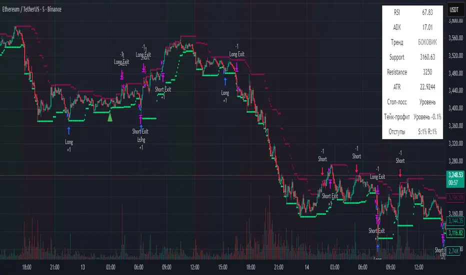
Fractional Candlestick Long Only Experimental V4 Another example of use an idea of Fractional Candlestick , based on mathematical rules of Fractional Calculus , typical kernel Caputo-Fabrizio ( CF ) and Atangana-Baleanu is used, alfa factor ( esential for calculation ) is in range 0,1-0.9.
Let's fun with this script .

KELTNER + ADX 전략It's a trend strategy based on the Keltner channel and ADX. It's optimized for the Bitcoin Futures 15 Distribution Chart.
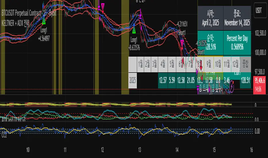
GMH : Tech Bubble Good Morning Holding
Simulating How to Ride the Bubble — and Jump Out Before the Crash
Be careful! Most simulation results show that this strategy sometimes underperforms a simple buy-and-hold, because it gives away positions during deep retracements and buys back at higher thresholds.
Humans often struggle with cutting losses. When the pain becomes too much, they lose the confidence needed to execute even a reasonable strategy.
But in terms of mentality, this approach reduces long-term portfolio volatility. It helps investors feel more at peace, especially during real market crashes like the tech bubble in 2021.
How to use : Select TimeFrame 4HR on trading view

Quasimodo Pattern Strategy Back Test [TradingFinder] QM Trading🔵 Introduction
The QM pattern, also known as the Quasimodo pattern, is one of the popular patterns in price action, and it is often used by technical analysts. The QM pattern is used to identify trend reversals and provides a very good risk-to-reward ratio. One of the advantages of the QM pattern is its high frequency and visibility in charts.
Additionally, due to its strength, it is highly profitable, and as mentioned, its risk-to-reward ratio is very good. The QM pattern is highly popular among traders in supply and demand, and traders also use this pattern.
The Price Action QM pattern, like other Price Action patterns, has two types: Bullish QM and Bearish QM patterns. To identify this pattern, you need to be familiar with its types to recognize it.
🔵 Identifying the QM Pattern
🟣 Bullish QM
In the bullish QM pattern, as you can see in the image below, an LL and HH are formed. As you can see, the neckline is marked as a dashed line. When the price reaches this range, it will start its upward movement.
🟣 Bearish QM
The Price Action QM pattern also has a bearish pattern. As you can see in the image below, initially, an HH and LL are formed. The neckline in this image is the dashed line, and when the LL is formed, the price reaches this neckline. However, it cannot pass it, and the downward trend resumes.
🔵 How to Use
The Quasimodo pattern is one of the clearest structures used to identify market reversals. It is built around the concept of a structural break followed by a pullback into an area of trapped liquidity. Instead of relying on lagging indicators, this pattern focuses purely on price action and how the market reacts after exhausting one side of liquidity. When understood correctly, it provides traders with precise entry points at the transition between trend phases.
🟣 Bullish Quasimodo
A bullish Quasimodo forms after a clear downtrend when sellers start losing control. The market continues to make lower lows until a sudden higher high appears, signaling that buyers are entering with strength. Price then pulls back to retest the previous low, creating what is known as the Quasimodo low.
This area often becomes the final trap for sellers before the market shifts upward. A visible rejection or displacement from this zone confirms bullish momentum. Traders usually place entries near this level, stops below the low, and targets at previous highs or the next resistance zone. Combining the setup with demand zones or Fair Value Gaps increases its accuracy.
🟣 Bearish Quasimodo
A bearish Quasimodo forms near the top of an uptrend when buyers begin to lose strength. The market continues to make higher highs until a sudden lower low breaks the bullish structure, showing that selling pressure is entering the market. Price then retraces upward to retest the previous high, forming the Quasimodo high, where breakout buyers are often trapped.
Once rejection appears at this level, it indicates a likely reversal. Traders can enter short near this area, with stop-losses placed above the high and targets near the next support or previous lows. The setup gains more reliability when aligned with supply zones, SMT divergence, or bearish Fair Value Gaps.
🔵 Setting
Pivot Period : You can use this parameter to use your desired period to identify the QM pattern. By default, this parameter is set to the number 5.
Take Profit Mode : You can choose your desired Take Profit in three ways. Based on the logic of the QM strategy, you can select two Take Profit levels, TP1 and TP2. You can also choose your take profit based on the Reward to Risk ratio. You must enter your desired R/R in the Reward to Risk Ratio parameter.
Stop Loss Refine : The loss limit of the QM strategy is based on its logic on the Head pattern. You can refine it using the ATR Refine option to prevent Stop Hunt. You can enter your desired coefficient in the Stop Loss ATR Adjustment Coefficient parameter.
Reward to Risk Ratio : If you set Take Profit Mode to R/R, you must enter your desired R/R here. For example, if your loss limit is 10 pips and you set R/R to 2, your take profit will be reached when the price is 20 pips away from your entry point.
Stop Loss ATR Adjustment Coefficient : If you set Stop Loss Refine to ATR Refine, you must adjust your loss limit coefficient here. For example, if your buy position's loss limit is at the price of 1000, and your ATR is 10, if you set Stop Loss ATR Adjustment Coefficient to 2, your loss limit will be at the price of 980.
Entry Level Validity : Determines how long the Entry level remains valid. The higher the level, the longer the entry level will remain valid. By default it is 2 and it can be set between 2 and 15.
🔵 Results
The following examples show the backtest results of the Quasimodo (QM) strategy in action. Each image is based on specific settings for the symbol, timeframe, and input parameters, illustrating how the QM logic can generate signals under different market conditions. The detailed configuration for each backtest is also displayed on the image.
⚠ Important Note : Even with identical settings and the same symbol, results may vary slightly across different brokers due to data feed variations and pricing differences.
Default Properties of Backtests :
OANDA:XAUUSD | TimeFrame: 5min | Duration: 1 Year :
BINANCE:BTCUSD | TimeFrame: 5min | Duration: 1 Year :
CAPITALCOM:US30 | TimeFrame: 5min | Duration: 1 Year :
NASDAQ:QQQ | TimeFrame: 5min | Duration: 5 Year :
OANDA:EURUSD | TimeFrame: 5min | Duration: 5 Year :
PEPPERSTONE:US500 | TimeFrame: 5min | Duration: 5 Year :

XAU/USD Weekly Volatility Strategy by WeTradeAIWeTradeAI - XAU/USD Weekly Volatility Strategy
This strategy is designed for Gold (XAU/USD) trading, leveraging a weekly market structure and volatility projection model. It dynamically identifies high-probability zones based on the prior week’s price action and adapts to intraday movement.
🔍 Core Logic:
Weekly High, Low & Midpoint: Defines structural balance for directional bias.
Projected Volatility Zones:
Green Zone: Upward projection from last week’s low.
Red Zone: Downward projection from last week’s high.
Half-Volatility Lines: Act as breakout or reversal triggers.
Monday Open: Serves as a temporary directional reference until midweek.
Daily High, Low, and Mid: Used for intraday stop-loss placement and validation.
🎯 Trade Entries:
Breakout Entries: Triggered when price breaks and holds above/below the Half-Vol levels.
Reversal Entries: Triggered by strong rejections near outer zones, reverting back toward equilibrium.
🛡️ Risk Management:
Dynamic Stop-Loss: Based on the previous day’s midpoint.
⏱️ Multi-Timeframe Usage:
4H – Weekly structure & context
1H – Trend alignment
15M – Precision entries

RastaRasta — Educational Strategy (Pine v5)
Momentum · Smoothing · Trend Study
Overview
The Rasta Strategy is a visual and educational framework designed to help traders study momentum transitions using the interaction between a fast-reacting EMA line and a slower smoothed reference line.
It is not a signal generator or profit system; it’s a learning tool for understanding how smoothing, crossovers, and filters interact under different market conditions.
The script displays:
A primary EMA line (the fast reactive wave).
A Smoothed line (using your chosen smoothing method).
Optional fog zones between them for quick visual context.
Optional DNA rungs connecting both lines to illustrate volatility compression and expansion.
Optional EMA 8 / EMA 21 trend filter to observe higher-time-frame alignment.
Core Idea
The Rasta model focuses on wave interaction. When the fast EMA crosses above the smoothed line, it reflects a shift in short-term momentum relative to background trend pressure. Cross-unders suggest weakening or reversal.
Rather than treating this as a trading “signal,” use it to observe structure, study trend alignment, and test how smoothing type affects reaction speed.
Smoothing Types Explained
The script lets you experiment with multiple smoothing techniques:
Type Description Use Case
SMA (Simple Moving Average) Arithmetic mean of the last n values. Smooth and steady, but slower. Trend-following studies; filters noise on higher time frames.
EMA (Exponential Moving Average) Weights recent data more. Responds faster to new price action. Momentum or reactive strategies; quick shifts and reversals.
RMA (Relative Moving Average) Used internally by RSI; smooths exponentially but slower than EMA. Momentum confirmation; balanced response.
WMA (Weighted Moving Average) Linear weights emphasizing the most recent data strongly. Intraday scalping; crisp but potentially noisy.
None Disables smoothing; uses the EMA line alone. Raw comparison baseline.
Each smoothing method changes how early or late the strategy reacts:
Faster smoothing (EMA/WMA) = more responsive, good for scalping.
Slower smoothing (SMA/RMA) = more stable, good for trend following.
Modes of Study
🔹 Scalper Mode
Use short EMA lengths (e.g., 3–5) and fast smoothing (EMA or WMA).
Focus on 1 min – 15 min charts.
Watch how quick crossovers appear near local tops/bottoms.
Fog and rung compression reveal volatility contraction before bursts.
Goal: study short-term rhythm and liquidity pulses.
🔹 Momentum Mode
Use moderate EMA (5–9) and RMA smoothing.
Ideal for 1 H–4 H charts.
Observe how the fog color aligns with trend shifts.
EMA 8 / 21 filter can act as macro bias; “Enter” labels will appear only in its direction when enabled.
Goal: study sustained motion between pullbacks and acceleration waves.
🔹 Trend-Follower Mode
Use longer EMA (13–21) with SMA smoothing.
Great for daily/weekly charts.
Focus on periods where fog stays unbroken for long stretches — these illustrate clear trend dominance.
Watch rung spacing: tight clusters often precede consolidations; wide rungs signal expanding volatility.
Goal: visualize slow-motion trend transitions and filter whipsaw conditions.
Components
EMA Line (Red): Fast-reacting short-term direction.
Smoothed Line (Yellow): Reference trend baseline.
Fog Zone: Green when EMA > Smoothed (up-momentum), red when below.
DNA Rungs: Thin connectors showing volatility structure.
EMA 8 / 21 Filter (optional):
When enabled, the strategy will only allow Enter events if EMA 8 > EMA 21.
Use this to study higher-trend gating effects.
Educational Applications
Momentum Visualization: Observe how the fast EMA “breathes” around the smoothed baseline.
Trend Transitions: Compare different smoothing types to see how early or late reversals are detected.
Noise Filtering: Experiment with fog opacity and smoothing lengths to understand trade-off between responsiveness and stability.
Risk Concept Simulation: Includes a simple fixed stop-loss parameter (default 13%) for educational demonstrations of position management in the Strategy Tester.
How to Use
Add to Chart → “Strategy.”
Works on any timeframe and instrument.
Adjust Parameters:
Length: base EMA speed.
Smoothing Type: choose SMA, EMA, RMA, or WMA.
Smoothing Length: controls delay and smoothness.
EMA 8 / 21 Filter: toggles trend gating.
Fog & Rungs: visual study options only.
Study Behavior:
Use Strategy Tester → List of Trades for entry/exit context.
Observe how different smoothing types affect early vs. late “Enter” points.
Compare trend periods vs. ranging periods to evaluate efficiency.
Combine with External Tools:
Overlay RSI, MACD, or Volume for deeper correlation analysis.
Use replay mode to visualize crossovers in live sequence.
Interpreting the Labels
Enter: Marks where fast EMA crosses above the smoothed line (or when filter flips positive).
Exit: Marks where fast EMA crosses back below.
These are purely analytical markers — they do not represent trade advice.
Educational Value
The Rasta framework helps learners explore:
Reaction time differences between moving-average algorithms.
Impact of smoothing on signal clarity.
Interaction of local and global trends.
Visualization of volatility contraction (tight DNA rungs) and expansion (wide fog zones).
It’s a sandbox for studying price structure, not a promise of profit.
Disclaimer
This script is provided for educational and research purposes only.
It does not constitute financial advice, trading signals, or performance guarantees. Past market behavior does not predict future outcomes.
Users are encouraged to experiment responsibly, record observations, and develop their own understanding of price behavior.
Author: Michael Culpepper (mikeyc747)
License: Educational / Open for study and modification with credit.
Philosophy:
“Learning the rhythm of the market is more valuable than chasing its profits.” — Rasta
