Universal Adaptive Tracking🙏🏻 Behold, this is UAT (Universal Adaptive Tracker) , with less words imma proceed how it compares with alternatives:
^^ comparison with non-adaptive quadratic regression (purple line), that has higher overshoots, less precision
^^ comparison with JMA and its adaptive gain. JMA’s gain is heavily limited, while UAT’s negative and positive gains are soft-saturated with p-order Möbius transform
This drop is inspired by, dedicated to, and made will all love towards Jurik Research , who retired in October 2k21. When some1 steps out, some1 has to step in, and that time it’s me (again xd). But there’s some history u gotta know:
Some history u gotta know:
In ~2008 dudes from forexfactory reverse engineered Jurik Moving Average
In late 1990s dudes from Jurik Research approximated the best possible adaptive tracking filter for evolution of prices via engineering miracles
Today in 2k26, me I'm gonna present to you the real mathematical objects/entities behind JMA top-edge engineered approximates. You will prolly be even more happy now then all the dem together back then.
Why all this?
When we talk about object tracking stuff, e.g. air defense, drones, missiles, projectiles, prices, etc, it all comes down to adaptive control and (Position & Velocity & Acceleration) aka PVA state space models (the real stuff many of you count as DSP ).
Why? Cuz while position (P) : (mean), or position & velocity (PV) : (linear regression) are stable enough in dem own ways, Position & Velocity & Acceleration (PVA) : (quadratic regression+) require adaptivity do be stable. And real world stuff needs PVA, due to non-linearity for starters.
So that’s why. If your goal is Really smoothing and no lag, u gotta go there. I see a lot of folks are crazy with it and want it, so here is it, for y’all. And good news, this is perfect for your favorite Moving Windows.
How to use it
The upper study:
The final filter (main state): just as you use other fast smoothers, MAs, etc, you know better than me here
You can also turn in volatility bands in script’s style settings, these do not require any adjustments
Finally, you can turn on, in the same place, separate trackers each based on negative and positive volatility exclusively. When both are almost equal, that indicates stability & persistence in markets. May sound like it’s nothing important, but I've never seen anything like it before. Also, if you'd allow your our inner mental gym hero gloriously arise, you can argue that these 2 separate trackers represent 2 fair prices (one for sellers, one for buyers). All better then 1 imaginary fair price for both (forget about it)
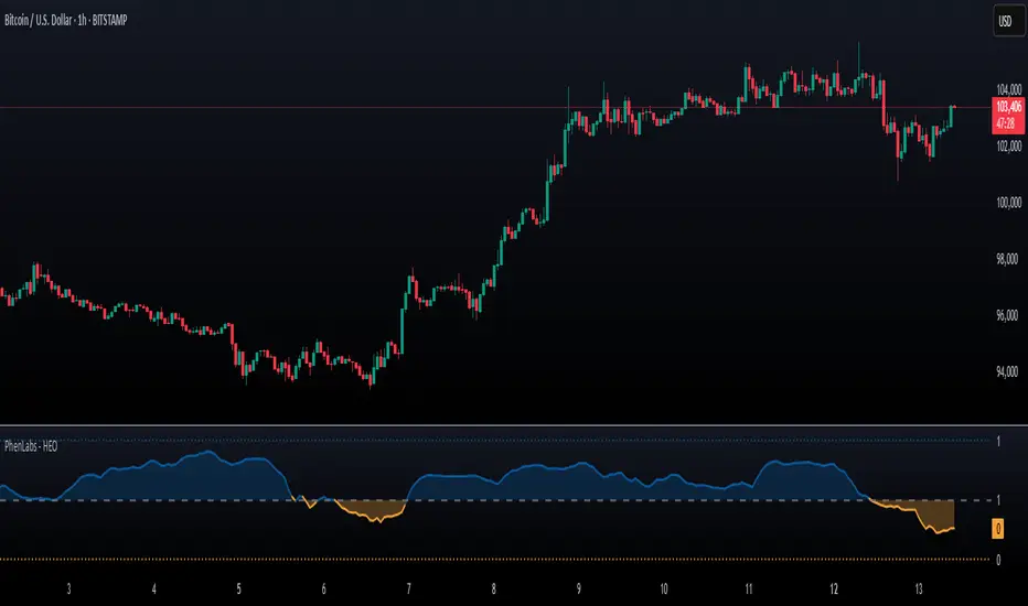
The lower study:
The lower study: you can analyze streams of upward of downward volatilities separately. This is incredibly powerful
You can also turn these off and turn on neg & pos intensities, and use them as trend detector, when each or both cross 1.5 (naturally neutral) threshold.
^^ Upper study with expected typical and maximum volatility bands turned On
...
The method explained
What you got in the end is non-linear, adaptive, lighting fast when needed and slow when required price tracking. All built upon real math entities/objects, not a brilliantly engineered approximation of them. No parameters to optimize, data tells it all.
... It all starts from a process model, in our cause this is...
MFPM (Mechanical Feedback Price Model)
Doesn’t make gaussian assumptions like most quant mainstream tech, accepts that innovations are Laplace “at best”, relies in L inf and L0 spaces.
I created this model neither trynna fit non-fitting ARMA / variants, nor trynna be silly assuming that price state evolution and markets are random.
Theory behind it: if no new volume comes, then price evolution would be simply guided by the feedback based on previous trading activity, pushing prices towards the midrange between 2 latest datapoints, being the main force behind so called “pullbacks” and reason why most pullbacks end just a bit past 50% of a move.
This is the Real mechanical feedback based mean reversion, that is always there in the markets no matter what, think of it as a background process that is always there, and fresh new volume deviates prices away from it. Btw, this can also be expressed as AR2 with both phis = 0.5 .
Then I separate positive and negative innovations from this model and process them separately, reflecting the asymmetry between buy and sell forces, smth that most forget. Both of these follow exponential distribution . Each stream has its own memory so here we use recursive operators . We track maximum innovations (differences between real and expected datapoints) with exponentially decaying damping factor, and keep tracking typical innovation, with the same factor.
Then we calculate what’s called in lovely audio engineering as “ crest factor ”, the difference is we don’t do RMS and stuff. But hey again we work with laplace innovations, so we keep things in L0 and L inf spirit. Then we go a couple of steps further, making this crest factor truly relative (resolution agnostic), and then, most importantly, we apply a natural saturation on it based on p-order Möbius transform, but not with arbitrary p and L, but guided by informational limits of the data. These final "intensity" parameters are what we need next to make our object tracking adaptive.
Extended Beta(2, 2) Window
This is imo the main part of this. Looking at tapering windows in DSP and how wavelets are made from derivatives of PDF functions of probability distributions, I figured that why use just one derivative? That made me come up with Universal Moving Average , that combines PDF and CDF of Beta(2, 2) distribution . And that is fine for P (position) tracking model.
Here we need PVA (position & velocity & acceleration). We can realize that everything starts from PDF, and by adding derivatives and anti-derivatives of it as factors of final window weights, we can create smth truly unique, a weightset that is non-arbitrary and naturally provides response alike quadratic regression does, But, naturally smoothed.
Why do I consider this a discovery, a primordial math object? Because x^2 itself and Beta(2, 2) based on it are the only primitives, esp out of all these dozens of DSP tapering windows, that provide you a finite amount of derivatives. You can keep differentiating Hann window until the kingdom f come, while Welch window aka Beta(2, 2) has a natural stopping point, because the 3rd derivative is 0, so we can’t use it. Symmetrically, we do 2 steps up from PDF, getting 1st and second anti-derivatives. What’s lovely, symmetrically, 3rd antiderivative even tho exist, it stops making any sense. 2nd one still makes sense, it’s smth like “potential” of probability distribution, not really discussed in mainstream open access sources.
Finally, the last part is to introduce adaptivity using these intensity exponents we’ve calculated with MFPM. We do 2 separate trackers, one using the negative intensity exponent, another one uses positive intensity exponent.
And at the end, even tho using both together is cool, the final state estimate is calculated simply as the state which intensity has higher.
^^ impulse response of our final kernel with fixed (non adaptive) intensity exponents: 1 (blue) and 2 (red). You see it's all about phase
…
And that’s all folks.
…
Actually no …
Last, not least, is the ability to add additional innovation weight to the kernel:
^^ Weighting by innovations “On”. Provides incredible tracking precision, paid with smoothness. I think this screenshot, showing what happened after the gap, and how the tracker managed to react, explains it all.
...
Live Long and Prosper, all good TradingView
∞
Nonlinear
Hurst Exponent Oscillator [PhenLabs]📊 Hurst Exponent Oscillator -
Version: PineScript™ v5
📌 Description
The Hurst Exponent Oscillator (HEO) by PhenLabs is a powerful tool developed for traders who want to distinguish between trending, mean-reverting, and random market behaviors with clarity and precision. By estimating the Hurst Exponent—a statistical measure of long-term memory in financial time series—this indicator helps users make sense of underlying market dynamics that are often not visible through traditional moving averages or oscillators.
Traders can quickly know if the market is likely to continue its current direction (trending), revert to the mean, or behave randomly, allowing for more strategic timing of entries and exits. With customizable smoothing and clear visual cues, the HEO enhances decision-making in a wide range of trading environments.
🚀 Points of Innovation
Integrates advanced Hurst Exponent calculation via Rescaled Range (R/S) analysis, providing unique market character insights.
Offers real-time visual cues for trending, mean-reverting, or random price action zones.
User-controllable EMA smoothing reduces noise for clearer interpretation.
Dynamic coloring and fill for immediate visual categorization of market regime.
Configurable visual thresholds for critical Hurst levels (e.g., 0.4, 0.5, 0.6).
Fully customizable appearance settings to fit different charting preferences.
🔧 Core Components
Log Returns Calculation: Computes log returns of the selected price source to feed into the Hurst calculation, ensuring robust and scale-independent analysis.
Rescaled Range (R/S) Analysis: Assesses the dispersion and cumulative deviation over a rolling window, forming the core statistical basis for the Hurst exponent estimate.
Smoothing Engine: Applies Exponential Moving Average (EMA) smoothing to the raw Hurst value for enhanced clarity.
Dynamic Rolling Windows: Utilizes arrays to maintain efficient, real-time calculations over user-defined lengths.
Adaptive Color Logic: Assigns different highlight and fill colors based on the current Hurst value zone.
🔥 Key Features
Visually differentiates between trending, mean-reverting, and random market modes.
User-adjustable lookback and smoothing periods for tailored sensitivity.
Distinct fill and line styles for each regime to avoid ambiguity.
On-chart reference lines for strong trending and mean-reverting thresholds.
Works with any price series (close, open, HL2, etc.) for versatile application.
🎨 Visualization
Hurst Exponent Curve: Primary plotted line (smoothed if EMA is used) reflects the ongoing estimate of the Hurst exponent.
Colored Zone Filling: The area between the Hurst line and the 0.5 reference line is filled, with color and opacity dynamically indicating the current market regime.
Reference Lines: Dash/dot lines mark standard Hurst thresholds (0.4, 0.5, 0.6) to contextualize the current regime.
All visual elements can be customized for thickness, color intensity, and opacity for user preference.
📖 Usage Guidelines
Data Settings
Hurst Calculation Length
Default: 100
Range: 10-300
Description: Number of bars used in Hurst calculation; higher values mean longer-term analysis, lower values for quicker reaction.
Data Source
Default: close
Description: Select which data series to analyze (e.g., Close, Open, HL2).
Smoothing Length (EMA)
Default: 5
Range: 1-50
Description: Length for smoothing the Hurst value; higher settings yield smoother but less responsive results.
Style Settings
Trending Color (Hurst > 0.5)
Default: Blue tone
Description: Color used when trending regime is detected.
Mean-Reverting Color (Hurst < 0.5)
Default: Orange tone
Description: Color used when mean-reverting regime is detected.
Neutral/Random Color
Default: Soft blue
Description: Color when market behavior is indeterminate or shifting.
Fill Opacity
Default: 70-80
Range: 0-100
Description: Transparency of area fills—higher opacity for stronger visual effect.
Line Width
Default: 2
Range: 1-5
Description: Thickness of the main indicator curve.
✅ Best Use Cases
Identifying if a market is regime-shifting from trending to mean-reverting (or vice versa).
Filtering signals in automated or systematic trading strategies.
Spotting periods of randomness where trading signals should be deprioritized.
Enhancing mean-reversion or trend-following models with regime-awareness.
⚠️ Limitations
Not predictive: Reflects current and recent market state, not future direction.
Sensitive to input parameters—overfitting may occur if settings are changed too frequently.
Smoothing can introduce lag in regime recognition.
May not work optimally in markets with structural breaks or extreme volatility.
💡 What Makes This Unique
Employs advanced statistical market analysis (Hurst exponent) rarely found in standard toolkits.
Offers immediate regime visualization through smart dynamic coloring and zone fills.
🔬 How It Works
Rolling Log Return Calculation:
Each new price creates a log return, forming the basis for robust, non-linear analysis. This ensures all price differences are treated proportionally.
Rescaled Range Analysis:
A rolling window maintains cumulative deviations and computes the statistical “range” (max-min of deviations). This is compared against the standard deviation to estimate “memory”.
Exponent Calculation & Smoothing:
The raw Hurst value is translated from the log of the rescaled range ratio, and then optionally smoothed via EMA to dampen noise and false signals.
Regime Detection Logic:
The smoothed value is checked against 0.5. Values above = trending; below = mean-reverting; near 0.5 = random. These control plot/fill color and zone display.
💡 Note:
Use longer calculation lengths for major market character study, and shorter ones for tactical, short-term adaptation. Smoothing balances noise vs. lag—find a best fit for your trading style. Always combine regime awareness with broader technical/fundamental context for best results.
Ehlers NonLinear Filter [CC]The NonLinear Filter was created by John Ehlers and this one of his more unknown filters that work very well as a trendline and moving average. This is one of my favorites along with the instantenous trendlines that he created. Buy when the line turns green and sell when it turns red.
Let me know if there are any other indicators you would like to see me publish scripts for!
Garch (1,1) ModelThe Garch (General Autoregressive Conditional Heteroskedasticity) model is a non-linear time series model that uses past data to forecast future variance.
The Garch (1,1) formula is:
Garch = (gamma * Long Run Variance) + (alpha * Squared Lagged Returns) + (beta * Lagged Variance)
The gamma, alpha, and beta values are all weights used in the Garch calculations. According to RiskMetrics by JP Morgan, the optimal beta weight is 0.94, but this figure is highly disputed in the academic realm. The biggest problem academics and economists have with the 0.94 figure is that JP Morgan used monthly data to come to this number, meaning it does not take other time frames into account. Because of the disputed nature of what beta should be, this script will automatically calculate the beta weight for you in real time, taking into account the time frame you're using and realized variance, by using the Minimum Sum of Squared Errors Method.
The gamma and alpha weights are also calculated for you.
Even though the Garch formula provides today's projected variance, today's projected deviation is also calculated. This is done by taking the square root of Garch.
Additionally, if you want to project the variance or deviation for as many days forward as you want, you can.
In order to project the variance and deviation beyond just today, these equations are used:
Projected Variance = Long Run Variance + (alpha + beta)^Days Forward * (Garch - Long Run Variance)
Projected Deviation = sqrt(Projected Variance)
How to use this model:
1st. Decide the type of data you want: Projected Variance in % or Projected Deviation in %.
2nd. Decide how many days you want projected forward. If you input 0, you will get projections for today. If you input 1, you will get projections for tomorrow, and etc.
That's it. If you have any further questions, I left detailed comments in the code explaining each step, as best as I could.


