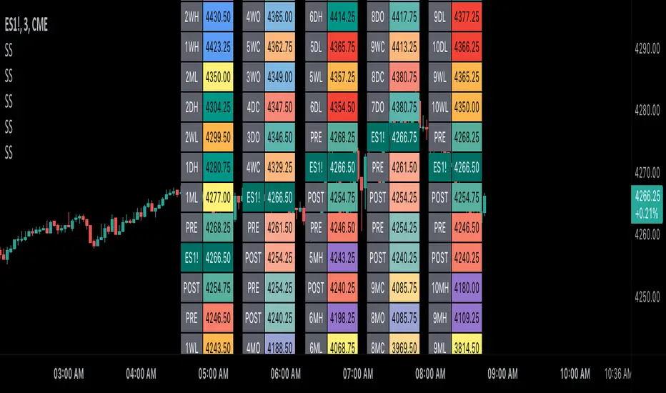
Scoopy StacksWaffle Around Multiple
(Open, High, Low, Close) Stacks On
Pre/Post Market & (Daily, Weekly,
Monthly, Yearly) Sessions With
Meticulous Columns, Rows, Tooltips,
Colors, Custom Ideas, and Alerts.
Sessions Use Two Step Incremental Values
Default Value: (1) Shows Two Previous
(O, H, L, C); Increasing Value Swaps
Sessions With Next Two Stacks.
⬛️ KEY WORDS:
🟢 Crossover | 🔴 Crossunder
📗 High | 📕 Low
📔 Open | 📓 Close
🥇 First Idea | 🥈 Second Idea
🥉 Third Idea | 🎖️ Fourth Idea
🟥 ALERTS:
Default Option: (Per Bar)
Alerts Once Conditions Are Met
(Bar Close) Alerts When Bar Closes
Default Option: (Reg)
Alerts During Regular Market
Trading Hours, (0930-1600)
(Ext) Alerts During Extended
Market Hours, (1600-0930)
(24/7) Alerts All Day
Optional Preferences:
Regular Alerts - Stocks
Extended Alerts - Futures
24/7 Alerts - Crypto
🟧 STACKS:
Default Value: (1)
Incremental Stack Value, Increasing Value
Swaps Sessions With the Next Two Stacks
(✓) Swap Stacks?
Pre/Post Market High/Lows,
1-2 Day High/Lows, 1-2 Week High/Lows,
1-2 Month High/Lows, 1-2 Year High/Lows
( ) Swap Stacks?
Pre/Post Market Open/Close,
1-2 Day Open/Close, 1-2 Week Open/Close,
1-2 Month Open/Close, 1-2 Year Open/Close
🟨 EXAMPLES:
Default Stack:
🟢 | 📗 Pre Market High (PRE) | 4600.00
🔴 | 📕 Post Market Low (POST) | 420.00
Optional: (Open)
🟢 | 📔 Post Market Open (POST) | 4400.00
Optional: (Close)
🔴 | 📓 Pre Market Close (PRE) | 430.00
Default Stack Value: (1)
🔴 | 📗 1 Day High (1DH) | 460.00
Next Stack Value: (3)
🟢 | 📕 4 Day Low (4DL) | 420.00
Optional: (Open)
🔴 | 📔 2 Day Open (2DO) | 440.00
Optional: (Close)
🟢 | 📓 3 Day Close (3DC) | 430.00
Default Stack Value: (5)
🟢 | 📗 5 Week High (5WH) | 460.00
Next Stack Value: (7)
🔴 | 📕 8 Week Low (8WL) | 420.00
Optional: (Open)
🔴 | 📔 7 Week Open (7WO) | 4400.00
Optional: (Close)
🟢 | 📓 6 Week Close (6WC) | 430.00
Default Stack Value: (9)
🔴 | 📗 9 Month High (9MH) | 460.00
Next Stack Value: (11)
🟢 | 📕 12 Month Low (12ML) | 420.00
Optional: (Open)
🟢 | 📔 11 Month Open (11MO) | 4400.00
Optional: (Close)
🔴 | 📓 10 Month Close (10MC) | 430.00
Default Stack Value: (13)
🟢 | 📗 13 Year High (13YH) | 460.00
Next Stack Value: (15)
🟢 | 📕 16 Year Low (16YL) | 420.00
Optional: (Open)
🔴 | 📔 15 Year Open (15YO) | 4400.00
Optional: (Close)
🔴 | 📓 14 Year Close (14YC) | 430.00
🟩 TABLES:
Default Value: (1)
Moves Table Up, Down, Left, or Right
Based on Second Default Value
First Default Value: (Top Right)
Sets Table Placement, Middle Center
Allows Table To Move In All Directions
Second Default Value: (Default)
Fixed Table Position, Switching Values
Moves Direction of the Table
🟦 IDEAS:
(✓) Show Ideas?
Shows Four Ideas With Custom Texts
and Values; Ideas Are Based Around
Post-It Note Reminders with Alerts
Suggestions For Text Ideas:
Take Profit, Stop Loss, Trim, Hold,
Long, Short, Bounce Spot, Retest,
Chop, Support, Resistance, Buy, Sell
🟪 EXAMPLES:
Default Value: (5)
Shows the Custom Table Value For
Sorted Table Positions and Alerts
Default Text: (🥇)
Shown On First Table Cell and
Message Appearing On Alerts
Alert Shows: 🟢 | 🥇 | 5.00
Default Value: (10)
Shows the Custom Table Value For
Sorted Table Positions and Alerts
Default Text: (🥈)
Shown On Second Table Cell and
Message Appearing On Alerts
Alert Shows: 🔴 | 🥈 | 10.00
Default Value: (50)
Shows the Custom Table Value For
Sorted Table Positions and Alerts
Default Text: (🥉)
Shown On Third Table Cell and
Message Appearing On Alerts
Alert Shows: 🟢 | 🥉 | 50.00
Default Value: (100)
Shows the Custom Table Value For
Sorted Table Positions and Alerts
Default Text: (🎖️)
Shown On Fourth Table Cell and
Message Appearing On Alerts
Alert Shows: 🔴 | 🎖️ | 100.00
⬛️ REFERENCES:
Pre-market Highs & Lows on regular
trading hours (RTH) chart
By Twingall
Previous Day Week Highs & Lows
By Sbtnc
Screener for 40+ instruments
By QuantNomad
Daily Weekly Monthly Yearly Opens
By Meliksah55
Tìm kiếm tập lệnh với "11月1日是什么星座"
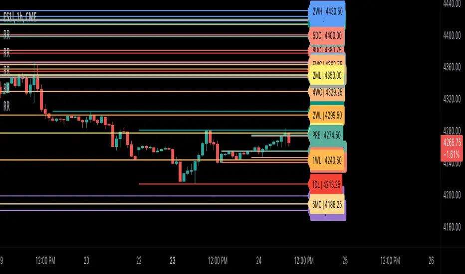
Ribbit RangesBounce Around Multiple
(Open, High, Low, Close) Ranges
On Pre/Post Market & (Daily, Weekly,
Monthly, Yearly) Sessions With
Meticulous Lines, Labels, Tooltips,
Colors, Custom Ideas, and Alerts.
Sessions Use Two Step Incremental Values
Default Value: (1) Shows Two Previous
(O, H, L, C); Increasing Value Swaps
Sessions With Next Two Ranges.
⬛️ KEY WORDS:
🟢 Crossover | 🔴 Crossunder
📗 High | 📕 Low
📔 Open | 📓 Close
🥇 First Idea | 🥈 Second Idea
🥉 Third Idea | 🎖️ Fourth Idea
🟥 ALERTS:
Default Option: (Per Bar)
Alerts Once Conditions Are Met
(Bar Close) Alerts When Bar Closes
Default Option: (Reg)
Alerts During Regular Market
Trading Hours, (0930-1600)
(Ext) Alerts During Extended
Market Hours, (1600-0930)
(24/7) Alerts All Day
Optional Preferences:
Regular Alerts - Stocks
Extended Alerts - Futures
24/7 Alerts - Crypto
🟧 RANGES:
Default Value: (1)
Incremental Range Value, Increasing Value
Swaps Sessions With the Next Two Ranges
(✓) Swap Ranges?
Pre/Post Market High/Lows,
1-2 Day High/Lows, 1-2 Week High/Lows,
1-2 Month High/Lows, 1-2 Year High/Lows
( ) Swap Ranges?
Pre/Post Market Open/Close,
1-2 Day Open/Close, 1-2 Week Open/Close,
1-2 Month Open/Close, 1-2 Year Open/Close
🟨 EXAMPLES:
Default Range:
🟢 | 📗 Pre Market High (PRE) | 4600.00
🔴 | 📕 Post Market Low (POST) | 420.00
Optional: (Open)
🟢 | 📔 Post Market Open (POST) | 4400.00
Optional: (Close)
🔴 | 📓 Pre Market Close (PRE) | 430.00
Default Range Value: (1)
🔴 | 📗 1 Day High (1DH) | 460.00
Next Range Value: (3)
🟢 | 📕 4 Day Low (4DL) | 420.00
Optional: (Open)
🔴 | 📔 2 Day Open (2DO) | 440.00
Optional: (Close)
🟢 | 📓 3 Day Close (3DC) | 430.00
Default Range Value: (5)
🟢 | 📗 5 Week High (5WH) | 460.00
Next Range Value: (7)
🔴 | 📕 8 Week Low (8WL) | 420.00
Optional: (Open)
🔴 | 📔 7 Week Open (7WO) | 4400.00
Optional: (Close)
🟢 | 📓 6 Week Close (6WC) | 430.00
Default Range Value: (9)
🔴 | 📗 9 Month High (9MH) | 460.00
Next Range Value: (11)
🟢 | 📕 12 Month Low (12ML) | 420.00
Optional: (Open)
🟢 | 📔 11 Month Open (11MO) | 4400.00
Optional: (Close)
🔴 | 📓 10 Month Close (10MC) | 430.00
Default Range Value: (13)
🟢 | 📗 13 Year High (13YH) | 460.00
Next Range Value: (15)
🟢 | 📕 16 Year Low (16YL) | 420.00
Optional: (Open)
🔴 | 📔 15 Year Open (15YO) | 4400.00
Optional: (Close)
🔴 | 📓 14 Year Close (14YC) | 430.00
🟩 COLORS:
(✓) Swap Colors?
Text Color Is Shown Using
Background Color
( ) Swap Colors?
Background Color Is Shown
Using Text Color
🟦 IDEAS:
(✓) Show Ideas?
Plots Four Ideas With Custom Lines
and Labels; Ideas Are Based Around
Post-It Note Reminders with Alerts
Suggestions For Text Ideas:
Take Profit, Stop Loss, Trim, Hold,
Long, Short, Bounce Spot, Retest,
Chop, Support, Resistance, Buy, Sell
🟪 EXAMPLES:
Default Value: (5)
Shows the Custom Value For
Lines, Labels, and Alerts
Default Text: (🥇)
Shown On First Label and
Message Appearing On Alerts
Alert Shows: 🟢 | 🥇 | 5.00
Default Value: (10)
Shows the Custom Value For
Lines, Labels, and Alerts
Default Text: (🥈)
Shown On Second Label and
Message Appearing On Alerts
Alert Shows: 🔴 | 🥈 | 10.00
Default Value: (50)
Shows the Custom Value For
Lines, Labels, and Alerts
Default Text: (🥉)
Shown On Third Label and
Message Appearing On Alerts
Alert Shows: 🟢 | 🥉 | 50.00
Default Value: (100)
Shows the Custom Value For
Lines, Labels, and Alerts
Default Text: (🎖️)
Shown On Fourth Label and
Message Appearing On Alerts
Alert Shows: 🔴 | 🎖️ | 100.00
⬛️ REFERENCES:
Pre-market Highs & Lows on regular
trading hours (RTH) chart
By Twingall
Previous Day Week Highs & Lows
By Sbtnc
Screener for 40+ instruments
By QuantNomad
Daily Weekly Monthly Yearly Opens
By Meliksah55
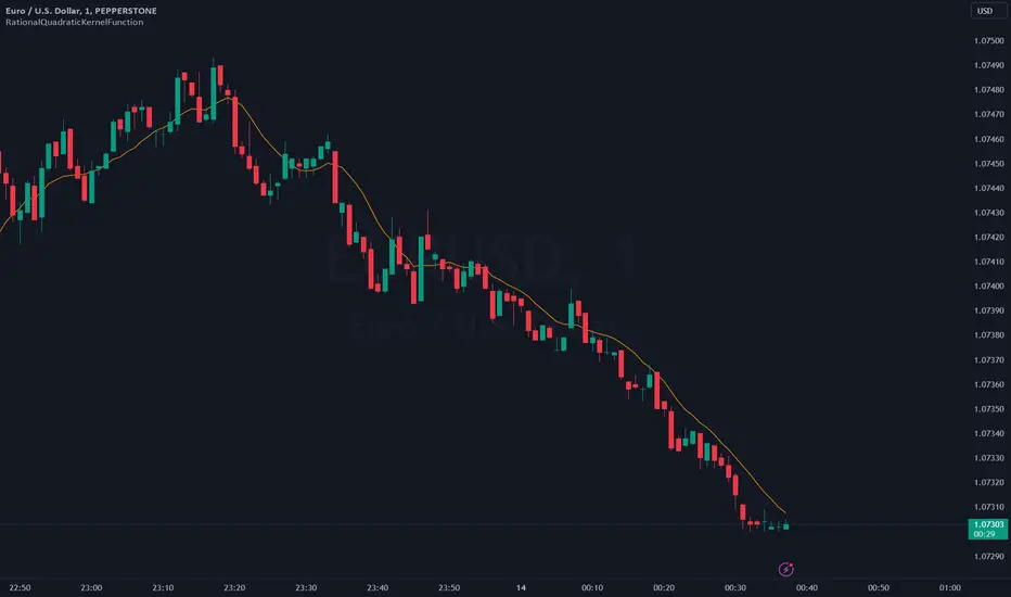
RationalQuadraticKernelFunctionDescription:
An optimised library for non-repainting Rational Quadratic Kernel Library. Added lookbackperiod and a validation to prevent division by zero.
Thanks to original author jdehorty.
Usage:
1. Import the library into your Pine Script code using the library function.
import vinayakavajiraya/RationalQuadraticKernelFunction/1
2. Call the Main Function:
Use the rationalQuadraticKernel function to calculate the Rational Quadratic Kernel estimate.
Provide the following parameters:
`_src` (series float): The input series of float values, typically representing price data.
`_lookback` (simple int): The lookback period for the kernel calculation (an integer).
`_relativeWeight` (simple float): The relative weight factor for the kernel (a float).
`startAtBar` (simple int): The bar index to start the calculation from (an integer).
rationalQuadraticEstimate = rationalQuadraticKernel(_src, _lookback, _relativeWeight, startAtBar)
3. Plot the Estimate:
Plot the resulting estimate on your TradingView chart using the plot function.
plot(rationalQuadraticEstimate, color = color.red, title = "Rational Quadratic Kernel Estimate")
Parameter Explanation:
`_src`: The input series of price data, such as 'close' or any other relevant data.
`_lookback`: The number of previous bars to consider when calculating the estimate. Higher values capture longer-term trends.
`_relativeWeight`: A factor that controls the importance of each data point in the calculation. A higher value emphasizes recent data.
`startAtBar`: The bar index from which the calculation begins.
Example Usage:
Here's an example of how to use the library to calculate and plot the Rational Quadratic Kernel estimate for the 'close' price series:
//@version=5
library("RationalQuadraticKernelFunctions", true)
rationalQuadraticEstimate = rationalQuadraticKernel(close, 11, 1, 24)
plot(rationalQuadraticEstimate, color = color.orange, title = "Rational Quadratic Kernel Estimate")
This example calculates the estimate for the 'close' price series, considers the previous 11 bars, assigns equal weight to all data points, and starts the calculation from the 24th bar. The result is plotted as an orange line on the chart.
Highly recommend to customize the parameters to suit your analysis needs and adapt the library to your trading strategies.
MOST + Moving Average ScreenerScreener version of Anıl Özekşi's Moving Stop Loss (MOST) Indicator:
USERS MAY SCREEN MOST WITH 11 DIFFERENT TYPES OF MOVING AVERAGES + THEY CAN ALSO SCREEN SIGNALS WITH THAT 11 MOVING AVERAGES INSTEAD OF USING MOST LINE.
Adjustable Moving Average Types:
SMA : Simple Moving Average
EMA : Exponential Moving Average
WMA : Weighted Moving Average
DEMA : Double Exponential Moving Average
TMA : Triangular Moving Average
VAR : Variable Index Dynamic Moving Average aka VIDYA
WWMA : Welles Wilder's Moving Average
ZLEMA : Zero Lag Exponential Moving Average
TSF : True Strength Force
HULL : Hull Moving Average
TILL : Tillson T3 Moving Average
About Screener Panel:
Users can explore 20 different and user-defined tickers, which can be changed from the SETTINGS (shares, crypto, commodities...) on this screener version.
The screener panel shows up right after the bars on the right side of the chart.
-In this screener version of MOST, users can define the number of demanded tickers (symbols) from 1 to 20 by checking the relevant boxes on the settings tab.
-All selected tickers can be screened in different timeframes.
-Also, different timeframes of the same Ticker can be screened.
IMPORTANT NOTICE:
Screener shows the results in 3 different logic:
1st LOGIC (Default Settings):
BUY AND SELL SIGNALS of MOST and MOVING AVERAGE LINE
Most Buy Signal: Moving Average Crosses ABOVE the MOST LINE
Most Sel Signal: Moving Average Crosses BELOW the MOST LINE
Tickers seen in green are the ones that are in an uptrend, according to MOST.
The ones that appear in red are those in the SELL signal, in a downtrend.
The numbers before each Ticker indicate how many bars passed after MOST's last BUY or SELL signal.
For example, according to the indicator, when BTCUSDT appears (3) in GREEN, Bitcoin switched to a BUY signal 3 bars ago.
2nd LOGIC (Moving Average & Price Flips Screener Mode):
This mode can only be activated by checking the 'Activate Moving Average Screening Mode' box on the settings menu.
MOST line will be disappeared after checking the box.
Buy Signal: When the Selected Price crosses ABOVE the selected Moving Average.
Sell Signal: When the Selected Price crosses BELOW the selected Moving Average.
Tickers seen in green are the ones that are in an uptrend, according to Moving Average & Price Flips.
The ones that appear in red are those in the SELL signal, in a downtrend.
The numbers before each Ticker indicate how many bars passed after the last BUY or SELL signal of Moving Average & Price Flips.
For example, according to the indicator, when BTCUSDT appears (3) in GREEN, Bitcoin switched to a BUY signal 3 bars ago.
3rd LOGIC (Moving Average Color Change Screener Mode):
Both 'Activate Moving Average Screening Mode' and 'Activate Moving Average Color Change Screening Mode' boxes must be checked in the settings tab.
Moving Average Line will turn out into two colors.
Green color means the moving average value is greater than the previous bar's value.
Red color means the moving average value is smaller than the previous bar's value.
Buy Signal: After the Selected Moving Average turns GREEN from red.
Sell Signal: After the Selected Moving Average turns RED from green.
-Screener shows the information about the color changes of the selected Moving Average with default settings.
If this option is preferred, users are advised to enlarge the length to have better signals.
Tickers seen in green are the ones that are in an uptrend, according to Moving Average Color.
The ones that appear in red are those in the SELL signal, in a downtrend.
The numbers before each Ticker indicate how many bars passed after the last BUY or SELL signal of Moving Average Color Change.
For example, according to the indicator, when BTCUSDT appears (3) in GREEN, Bitcoin switched to a BUY signal 3 bars ago.

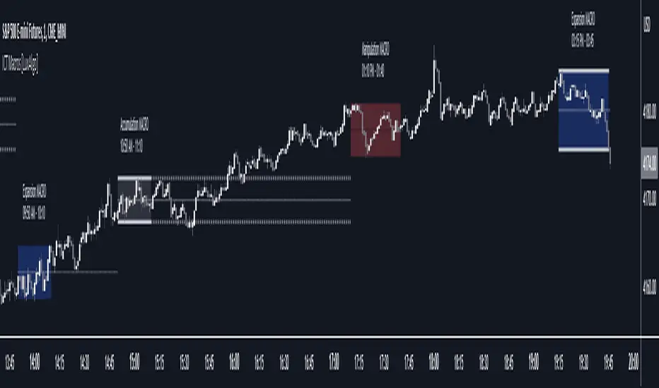
ICT Macros [LuxAlgo]The ICT Macros indicator aims to highlight & classify ICT Macros, which are time intervals where algorithmic trading takes place to interact with existing liquidity or to create new liquidity.
🔶 SETTINGS
🔹 Macros
Macro Time options (such as '09:50 AM 10:10'): Enable specific macro display.
Top Line , Mid Line , Bottom Line and Extending Lines options: Controls the lines for the specific macro.
🔹 Macro Classification
Length : A length to detect Market Structure Brakes and classify macro type based on detection.
Swing Area : Swing or Liquidity Area selection, highest/lowest of the wick or the candle bodies.
Accumulation , Manipulation and Expansion color options for the classified macros.
🔹 Others
Macro Texts : Controls both the size and the visibility of the macro text.
Alert Macro Times in Advance (Minutes) : This option will plot a vertical line presenting the start of the next macro time. The line will not appear all the time, but it will be there based on remaining minutes specified in the option.
Daylight Saving Time (DST) : Adjust time appropriate to Daylight Saving Time of the specific region.
🔶 USAGE
A macro is a way to automate a task or procedure which you perform on a regular basis.
In the context of ICT's teachings, a macro is a small program or set of instructions that unfolds within an algorithm, which influences price movements in the market. These macros operate at specific times and can be related to price runs from one level to another or certain market behaviors during specific time intervals. They help traders anticipate market movements and potential setups during specific time intervals.
To trade these effectively, it is important to understand the time of day when certain macros come into play, and it is strongly advised to introduce the concept of liquidity in your analysis.
Macros can be classified into three categories where the Macro classification is calculated based on the Market Structure prior to macro and the Market Structure during the macro duration:
Manipulation Macro
Manipulation macros are characterized by liquidity being swept both on the buyside and sellside.
Expansion Macro
Expansion macros are characterized by liquidity being swept only on the buyside or sellside. Prices within these macros are highly correlated with the overall trend.
Accumulation Macro
Accumulation macros are characterized by an accumulation of liquidity. Prices within these macros tend to range.
The script returns the maximum/minimum price values reached during the macro interval alongside the average between the maximum/minimum and extends them until a new macro starts. These levels can act as supports and resistances.
🔶 DETAILS
All required data for the macro detection and classification is retrieved using 1 minute data sets, this includes candles as well as pivot/swing highs and lows. This approach guarantees the visually presented objects are same (same highs/lows) on higher timeframes as well as the macro classification remain same as it is in 1 min charts.
8 Macros can be displayed by the script (4 are enabled by default):
02:33 AM 03:00 London Macro
04:03 AM 04:30 London Macro
08:50 AM 09:10 New York Macro
09:50 AM 10:10 New York Macro
10:50 AM 11:10 New York Macro
11:50 AM 12:10 New York Launch Macro
13:10 PM 13:40 New York Macro
15:15 PM 15:45 New York Macro
🔶 ALERTS
When an alert is configured, the user will have the ability to be notified in advance of the next Macro time, where the value specified in 'Alert Macro Times in Advance (Minutes)' option indicates how early to be notified.
🔶 LIMITATIONS
The script is supported on 1 min, 3 mins and 5 mins charts.
🔶 RELATED SCRIPTS
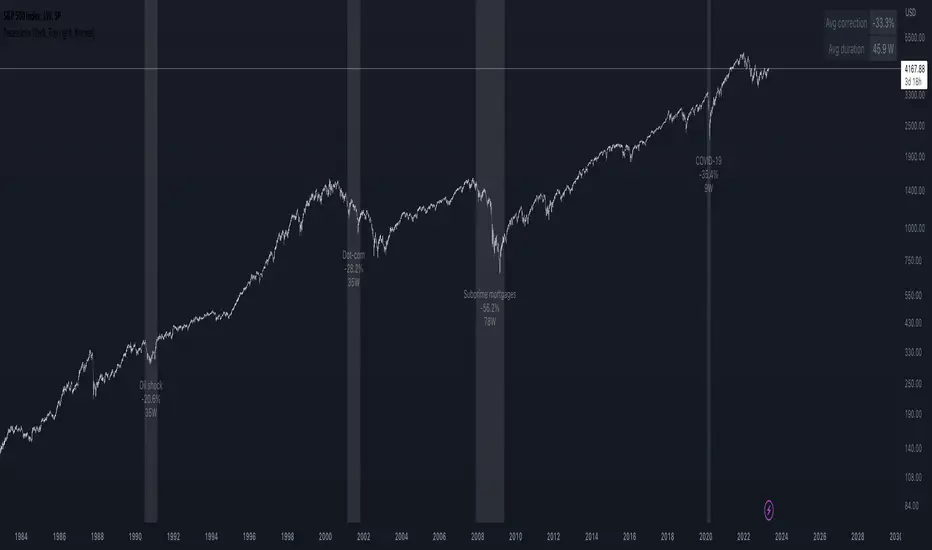
Recessions & crises shading (custom dates & stats)Shades your chart background to flag events such as crises or recessions, in similar fashion to what you see on FRED charts. The advantage of this indicator over others is that you can quickly input custom event dates as text in the menu to analyse their impact for your specific symbol. The script automatically labels, calculates and displays the peak to through percentage corrections on your current chart.
By default the indicator is configured to show the last 6 US recessions. If you have custom events which will benefit others, just paste the input string in the comments below so one can simply copy/paste in their indicator.
Example event input (No spaces allowed except for the label name. Enter dates as YYYY-MM-DD.)
2020-02-01,2020-03-31,COVID-19
2007-12-01,2009-05-31,Subprime mortgages
2001-03-01,2001-10-30,Dot-com bubble
1990-07-01,1991-03-01,Oil shock
1981-07-01,1982-11-01,US unemployment
1980-01-01,1980-07-01,Volker
1973-11-01,1975-03-01,OPEC
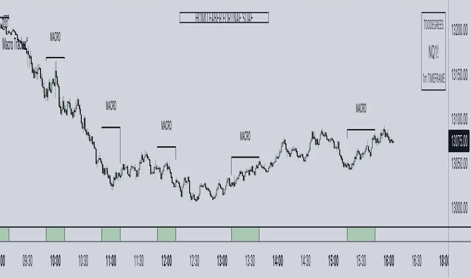
ICT Algorithmic Macro Tracker° (Open-Source) by toodegreesDescription:
The ICT Algorithmic Macro Tracker° Indicator is a powerful tool designed to enhance your trading experience by clearly and efficiently plotting the known ICT Macro Times on your chart.
Based on the teachings of the Inner Circle Trader , these Time windows correspond to periods when the Interbank Price Delivery Algorithm undergoes a series of checks ( Macros ) and is probable to move towards Liquidity.
The indicator allows traders to visualize and analyze these crucial moments in NY Time:
- 2:33-3:00
- 4:03-4:30
- 8:50-9:10
- 9:50-10:10
- 10:50-11:10
- 11:50-12:10
- 13:10-13:50
- 15:15-15:45
By providing a clean and clutter-free representation of ICT Macros, this indicator empowers traders to make more informed decisions, optimize and build their strategies based on Time.
Massive shoutout to @reastruth for his ICT Macros Indicator , and for allowing to create one of my own, go check him out!
Indicator Features:
– Track ongoing ICT Macros to aid your Live analysis.
- Gain valuable insights by hovering over the plotted ICT Macros to reveal tooltips with interval information.
– Plot the ICT Macros in one of two ways:
"On Chart": visualize ICT Macro timeframes directly on your chart, with automatic adjustments as Price moves.
Pro Tip: toggle Projections to see exactly where Macros begin and end without difficulty.
"New Pane": move the indicator two a New Pane to see both Live and Upcoming Macro events with ease in a dedicated section
Pro Tip: this section can be collapsed by double-clicking on the main chart, allowing for seamless trading preparation.
This indicator is available only on the TradingView platform.
⚠️ Open Source ⚠️
Coders and TV users are authorized to copy this code base, but a paid distribution is prohibited. A mention to the original author is expected, and appreciated.
⚠️ Terms and Conditions ⚠️
This financial tool is for educational purposes only and not financial advice. Users assume responsibility for decisions made based on the tool's information. Past performance doesn't guarantee future results. By using this tool, users agree to these terms.
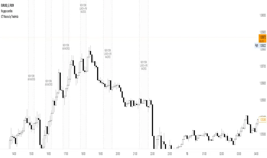
ICT Macros by CryptoforICT Macros by Cryptofor
Time periods in which the price is most volatile. At this time, the algorithm is programmed to attack liquidity or fill a significant FVG from which the OF can continue.
Plots of macros:
1. London Macros:
02:33 - 03:00
04:03 - 04:30
2. New York AM Macros:
08:50 - 09:10
09:50 - 10:10
10:50 - 11:10
3. New York Lunch + PM Macros:
11:50 - 12:10
13:10 - 13:40
15:15 - 15:45
Features:
Flexible line settings
Flexible text settings
Display data for all time or for the last 24 hours
Switch for each type of macro
Macro background color settings
TOMMAR#TOMMAR #MultiMovingAverages #MMAR
Dear fellow traders, this is Tommy, and today I'd like to introduce you to the Multi-Moving Averages Ribbon (MMAR) indicator, which I believe to be one of the best MMAR indicators available on TradingView. Moving Averages is a popular technical analysis tool used to smooth out price data by creating an average of past price data points over a specified time period. They can be used to identify trends and provide a clearer view of price action, as well as generate buy and sell signals by observing crossovers between different moving average lines.
In the MMAR indicator, we have incorporated 12 different types of Moving Averages, including Simple Moving Averages (SMA), Exponential Moving Averages (EMA), Weighted Moving Averages (WMA), Hull Moving Averages (HMA), and Smoothed Moving Averages (SMMA), among others. This allows traders to choose the optimal type for their preferred trading commodities.
One common technique in technical analysis is using multiple Moving Averages with varying lengths, which provides a more comprehensive view of price action. By analyzing multiple Moving Averages with different timeframes, traders can better understand both short- and long-term trends and make more informed trading decisions. Some of the well-known combinations of multiple moving averages used by traders are (5, 9, 14, 21, 45), (6, 11, 16, 22, 51), [8, 13, 21, 55), (50, 100, 200), and (60, 120, 240).
Another way to gauge the strength of the market trend is to look for the arrangement of the Moving Averages. If they are in a sequential order, with the shortest on top and the longest on the bottom, it is most likely a bullish trend. On the other hand, if they are arranged in reverse order, with the shortest on the bottom and the longest on top, it is most likely a bearish trend. The 'Trend Light' in the indicator settings will automatically signal when the Moving Averages are in either an orderly or reverse arrangement.
Lastly, I have added a useful feature to the indicator: the 'MA Projection'. This feature projects and forecasts the Moving Averages in the future, allowing traders to easily identify confluence zones in future candlesticks. Please note that the projection levels may change in the case of extreme price action that significantly affects the Moving Averages.
This is free so any Tradingview users can use this indicator. Just search TOMMAR in the indicator section located on top of the chart.
#TOMMAR #MultiMovingAverages #MMAR
안녕하세요 트레이더 여러분, 토미입니다. 오늘 여러분들에게 소개드릴 지표는 다양한 길이의 이동평균선 조합을 사용할 수 있는 MMAR (Multiple Moving Averages Ribbon)입니다. 아마 제가 만든 MMAR 지표가 트레이딩뷰에서 가장 쓸만할 겁니다. 이동평균선, 줄여서 이평선은 말 그대로 특정 기간 범위 내의 주가들을 평균한 값들로 이루어진 선입니다. 제가 이평선 관련된 강의 자료는 예전에 올려드린 바 있으니 더 자세한 내용이 궁금하신 분들은 아래 링크/이미지 클릭하시길 바랍니다.
본 지표는 Simple Moving Averages (SMA), Exponential Moving Averages (EMA), Weighted Moving Averages (WMA), Hull Moving Averages (HMA), 그리고 Smoothed Moving Averages (SMMA) 등을 포함해 총 12개 종류의 이평선 지표를 사용할 수 있습니다. 또한 각 이평선의 길이들도 하나하나 일일이 설정하실 수 있습니다. 예를 들어 요즘에 자주 보이는 이평선들의 조합이 , , , , 그리고 등등이 존재하는데 여러분의 취향에 맞게 설정하여 사용하시면 됩니다.
몇 가지 주요 기능에 대해서 설명 드리겠습니다. 설정에서 ‘Trend Light’를 키면 이평선들의 정배열 혹은 역배열 여부를 쉽게 볼 수 있습니다. 이평선이 정배열일때는 맨 아래의 이평선에 초록불이, 역배열일때는 맨 위의 이평선에 빨간불이 켜지며 둘 다 아닐 땐 아무 불도 켜지지 않습니다. 또한 ‘MA Projection’을 키면 이평선들의 미래 예측 값들을 확장해줍니다. 당연히 가격 변동이 갑자기 크게 나오면 이평선 예측 확장 레벨들이 확 바뀌겠죠.
지표창에 TOMMAR 검색하시거나 아래 즐겨찾기 인디케이터에 넣기 클릭하시면 누구나 사용하실 수 있습니다~ 여러분의 구독, 좋아요, 댓글은 저에게 큰 힘이 됩니다.

dmn's ICT ToolkitThis is my quality of life indicator for forex trading using the methods and concepts of ICT.
The idea is to automate marking up important price levels and times of the day instead of doing it manually every day.
Killzones
Marks the most volatile times of the day on the chart, during which the intraday high/low usually takes place.
Particularly impactful when there's news released during these times.
London Open (02:00-05:00 EST)
New York Open (08:30-11:00 EST)
London Close (10:00-11:30 EST)
True Day delineation
Vertical line at the start of the "true day" (00:00 EST), start of the algorithmic trading day and aids in visualizing the intraday direction.
New York midnight price level
Noteworthy price level at the start of the "true day".
This price level is referenced by the interbank trading algorithms during the day. Buy below it on bullish days, sell above it on bearish days.
Daily open price level
Reference level for optimal trade entries. Buy below it on bullish days, sell above it on bearish days.
Central Banks Dealers Range (CBDR) (14:00-20:00 EST) &
Central Banks Dealers Flout (CBDF) (15:00-24:00 EST) &
Asian Range (AR) (20:00-24:00 EST)
The standard deviation lines available are used to make predictions for short-term future highs/lows when the CBDR and AR are smaller than 40 pips.
Trade them by looking for 5/15min key levels that converge with the projection levels.
X days Average Daily Range (ADR)
Default to 5 days back, gives an idea of how much movement to expect intraday when the ADR high/low is converging with CBDR/CBDF/AR standard deviations.
Current Daily Range (CDR)
Used for comparison against the ADR to help determine if there's enough intraday range left to enter a trade.
Dynamically changes color based on percentage of the ADR. Green below 50% of ADR, orange between 50 and 100%, red when CDR exceeds ADR.
All of the above are used in conjunction with each other and higher timeframe levels of importance to find entries and target.
Note: Preferably use New York's time zone for your charts.

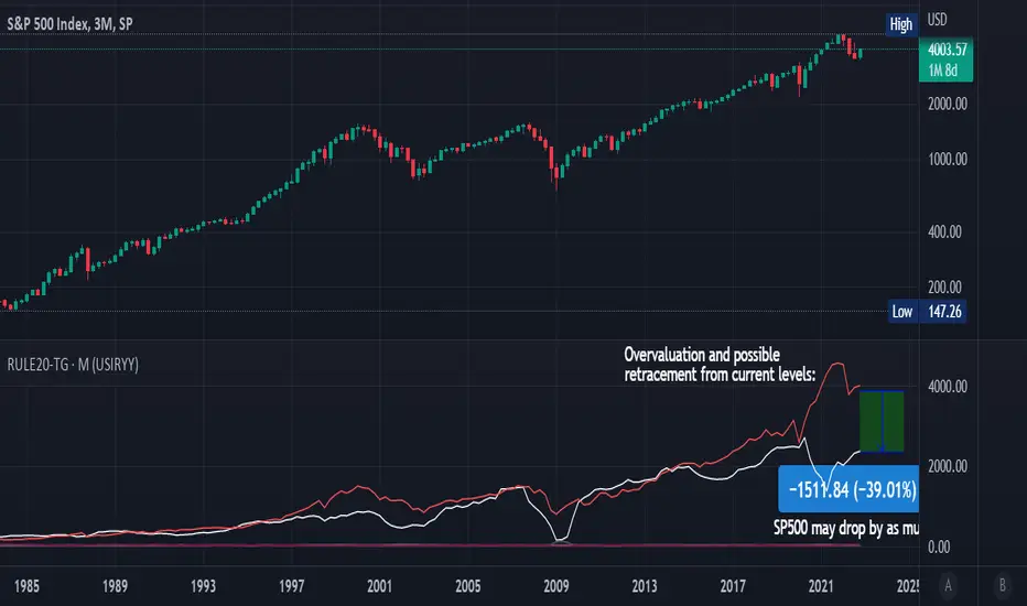
Rule Of 20 - Fair Value Estimation by Inflation & Earnings (TG)The Rule Of 20 is a heuristic calculation to find the fair value of an asset or market given its earnings and current inflation.
Its calculation is straightforward: the fair multiple of the price or price-to-earnings ratio of a stock should be 20 minus the rate of inflation.
In math terms: fair_price-to-earnings_ratio = (20 - inflation) ; fair_value = current_price * fair_price-to-earnings_ratio / real_price-to-earnings_ratio
For example, if a stock or index was trading on 11 times earnings and inflation was 2%, then the theory would be that the fair price-to-earnings ratio would be 20-2 = 18, which is much higher than the real price-to-earnings ratio of 11, and hence the asset would be undervalued.
Conversely, a market or company that was trading on 18 times price-to-earnings ration when inflation was 8% was seen as overvalued, because of the fair price-to-earnings ratio being 20-8=12, hence much lower than the real price-to-earnings ratio of 18.
We can then project the delta between the fair PE and real PE onto the asset's value to obtain the projected fair value, which may be a target of future value the asset may reach or hover around.
For example, as of 1st November 2022, SPX stood at 3871.97, with a PE ratio of 20.14 and an inflation in the US of 7.70. Using the Rule Of 20, we find that the fair PE ratio is 20-7.7=12.3, which is much lower than the current PE ratio of 20.14 by 39%! This may indicate a future possibility of a further downside risk by 39% from current valuation levels.
The origins of this rule are unknown, although the legendary US fund manager Peter Lynch is said to have been an active proponent when he was directing the Fidelity’s Magellan fund from 1977 to 1990.
For more infos about the Rule Of 20, reading this article is recommended: www.sharesmagazine.co.uk
This indicator implements the Rule Of 20 on any asset where the Financials are availble to TradingView, and also for the entire SP:SPX index as a way to assess the wider US stock market. Technically, the calculation is a bit different for the latter, as we cannot access earnings of SPX through Financials on TradingView, so we access it using the QUANDL:MULTPL/SP500_PE_RATIO_MONTH ticker instead.
By default are displayed:
current asset value in red
fair asset value according to the Rule Of 20 in white for SPX, or different shades of purple/maroon for other assets. Note that for SPX there is only one calculation, whereas for other assets there are multiple different ways to calculate earnings, so different fair values can be computed.
fair price-to-earnings ratio (PE ratio) in light grey.
real price-to-earnings ratio in darker grey.
This indicator can be used on SP:SPX ticker, and on most NASDAQ:* tickers, since they have Financials integrated in TradingView. Stocks tickers from other exchanges may not provide Financials data, so this indicator won't work then. If this happens, try to find the same ticker on NASDAQ instead.
Note that by default, only the US stock market is considered. If you want to consider stocks or assets in other regions of the world, please change the inflation ticker to a ticker that reflect the target region's inflation.
Also adding a table to ease interpretation was considered, but then the Timeframe MTF parameter would not work, and since the big advantage of this indicator is to allow for historical comparisons, the table was dropped.
Enjoy, and keep in mind that all models are wrong, but some are useful.
Trade safely!
TG
Centered Moving AverageThe Centered moving averages tries to resolve the problem that simple moving average are still not able to handle significant trends when forecasting.
When computing a running moving average in a centered way, placing the average in the middle time period makes sense.
If we average an even number of terms, we need to smooth the smoothed values.
Try to describe it with an example:
The following table shows the results using a centered moving average of 4.
nterim Steps
Period Value SMA Centered
1 9
1.5
2 8
2.5 9.5
3 9 9.5
3.5 9.5
4 12 10.0
4.5 10.5
5 9 10.750
5.5 11.0
6 12
6.5
7 11
This is the final table:
Period Value Centered MA
1 9
2 8
3 9 9.5
4 12 10.0
5 9 10.75
6 12
7 11
With this script we are able to process and display the centered moving average as described above.
In addition to this, however, the script is also able to estimate the potential projection of future data based on the available data by replicating where necessary the data of the last bar until the number of data necessary for the calculation of the required centered moving average is reached.
If for example I have 20 daily closings and I look for the moving average centered at 10, I receive the first data on the fifth day and the last data on the fourteenth day, so I have 5 days left uncovered, to remedy this I have to give the last value to the uncovered data the closing price of the last day.
The deviations work like the bollinger bands but must refer to the centered moving average.

STD-Adaptive T3 [Loxx]STD-Adaptive T3 is a standard deviation adaptive T3 moving average filter. This indicator acts more like a trend overlay indicator with gradient coloring.
What is the T3 moving average?
Better Moving Averages Tim Tillson
November 1, 1998
Tim Tillson is a software project manager at Hewlett-Packard, with degrees in Mathematics and Computer Science. He has privately traded options and equities for 15 years.
Introduction
"Digital filtering includes the process of smoothing, predicting, differentiating, integrating, separation of signals, and removal of noise from a signal. Thus many people who do such things are actually using digital filters without realizing that they are; being unacquainted with the theory, they neither understand what they have done nor the possibilities of what they might have done."
This quote from R. W. Hamming applies to the vast majority of indicators in technical analysis . Moving averages, be they simple, weighted, or exponential, are lowpass filters; low frequency components in the signal pass through with little attenuation, while high frequencies are severely reduced.
"Oscillator" type indicators (such as MACD , Momentum, Relative Strength Index ) are another type of digital filter called a differentiator.
Tushar Chande has observed that many popular oscillators are highly correlated, which is sensible because they are trying to measure the rate of change of the underlying time series, i.e., are trying to be the first and second derivatives we all learned about in Calculus.
We use moving averages (lowpass filters) in technical analysis to remove the random noise from a time series, to discern the underlying trend or to determine prices at which we will take action. A perfect moving average would have two attributes:
It would be smooth, not sensitive to random noise in the underlying time series. Another way of saying this is that its derivative would not spuriously alternate between positive and negative values.
It would not lag behind the time series it is computed from. Lag, of course, produces late buy or sell signals that kill profits.
The only way one can compute a perfect moving average is to have knowledge of the future, and if we had that, we would buy one lottery ticket a week rather than trade!
Having said this, we can still improve on the conventional simple, weighted, or exponential moving averages. Here's how:
Two Interesting Moving Averages
We will examine two benchmark moving averages based on Linear Regression analysis.
In both cases, a Linear Regression line of length n is fitted to price data.
I call the first moving average ILRS, which stands for Integral of Linear Regression Slope. One simply integrates the slope of a linear regression line as it is successively fitted in a moving window of length n across the data, with the constant of integration being a simple moving average of the first n points. Put another way, the derivative of ILRS is the linear regression slope. Note that ILRS is not the same as a SMA ( simple moving average ) of length n, which is actually the midpoint of the linear regression line as it moves across the data.
We can measure the lag of moving averages with respect to a linear trend by computing how they behave when the input is a line with unit slope. Both SMA (n) and ILRS(n) have lag of n/2, but ILRS is much smoother than SMA .
Our second benchmark moving average is well known, called EPMA or End Point Moving Average. It is the endpoint of the linear regression line of length n as it is fitted across the data. EPMA hugs the data more closely than a simple or exponential moving average of the same length. The price we pay for this is that it is much noisier (less smooth) than ILRS, and it also has the annoying property that it overshoots the data when linear trends are present.
However, EPMA has a lag of 0 with respect to linear input! This makes sense because a linear regression line will fit linear input perfectly, and the endpoint of the LR line will be on the input line.
These two moving averages frame the tradeoffs that we are facing. On one extreme we have ILRS, which is very smooth and has considerable phase lag. EPMA has 0 phase lag, but is too noisy and overshoots. We would like to construct a better moving average which is as smooth as ILRS, but runs closer to where EPMA lies, without the overshoot.
A easy way to attempt this is to split the difference, i.e. use (ILRS(n)+EPMA(n))/2. This will give us a moving average (call it IE /2) which runs in between the two, has phase lag of n/4 but still inherits considerable noise from EPMA. IE /2 is inspirational, however. Can we build something that is comparable, but smoother? Figure 1 shows ILRS, EPMA, and IE /2.
Filter Techniques
Any thoughtful student of filter theory (or resolute experimenter) will have noticed that you can improve the smoothness of a filter by running it through itself multiple times, at the cost of increasing phase lag.
There is a complementary technique (called twicing by J.W. Tukey) which can be used to improve phase lag. If L stands for the operation of running data through a low pass filter, then twicing can be described by:
L' = L(time series) + L(time series - L(time series))
That is, we add a moving average of the difference between the input and the moving average to the moving average. This is algebraically equivalent to:
2L-L(L)
This is the Double Exponential Moving Average or DEMA , popularized by Patrick Mulloy in TASAC (January/February 1994).
In our taxonomy, DEMA has some phase lag (although it exponentially approaches 0) and is somewhat noisy, comparable to IE /2 indicator.
We will use these two techniques to construct our better moving average, after we explore the first one a little more closely.
Fixing Overshoot
An n-day EMA has smoothing constant alpha=2/(n+1) and a lag of (n-1)/2.
Thus EMA (3) has lag 1, and EMA (11) has lag 5. Figure 2 shows that, if I am willing to incur 5 days of lag, I get a smoother moving average if I run EMA (3) through itself 5 times than if I just take EMA (11) once.
This suggests that if EPMA and DEMA have 0 or low lag, why not run fast versions (eg DEMA (3)) through themselves many times to achieve a smooth result? The problem is that multiple runs though these filters increase their tendency to overshoot the data, giving an unusable result. This is because the amplitude response of DEMA and EPMA is greater than 1 at certain frequencies, giving a gain of much greater than 1 at these frequencies when run though themselves multiple times. Figure 3 shows DEMA (7) and EPMA(7) run through themselves 3 times. DEMA^3 has serious overshoot, and EPMA^3 is terrible.
The solution to the overshoot problem is to recall what we are doing with twicing:
DEMA (n) = EMA (n) + EMA (time series - EMA (n))
The second term is adding, in effect, a smooth version of the derivative to the EMA to achieve DEMA . The derivative term determines how hot the moving average's response to linear trends will be. We need to simply turn down the volume to achieve our basic building block:
EMA (n) + EMA (time series - EMA (n))*.7;
This is algebraically the same as:
EMA (n)*1.7-EMA( EMA (n))*.7;
I have chosen .7 as my volume factor, but the general formula (which I call "Generalized Dema") is:
GD (n,v) = EMA (n)*(1+v)-EMA( EMA (n))*v,
Where v ranges between 0 and 1. When v=0, GD is just an EMA , and when v=1, GD is DEMA . In between, GD is a cooler DEMA . By using a value for v less than 1 (I like .7), we cure the multiple DEMA overshoot problem, at the cost of accepting some additional phase delay. Now we can run GD through itself multiple times to define a new, smoother moving average T3 that does not overshoot the data:
T3(n) = GD ( GD ( GD (n)))
In filter theory parlance, T3 is a six-pole non-linear Kalman filter. Kalman filters are ones which use the error (in this case (time series - EMA (n)) to correct themselves. In Technical Analysis , these are called Adaptive Moving Averages; they track the time series more aggressively when it is making large moves.
Included
Bar coloring
Loxx's Expanded Source Types

Softmax Normalized T3 Histogram [Loxx]Softmax Normalized T3 Histogram is a T3 moving average that is morphed into a normalized oscillator from -1 to 1.
What is the Softmax function?
The softmax function, also known as softargmax: or normalized exponential function, converts a vector of K real numbers into a probability distribution of K possible outcomes. It is a generalization of the logistic function to multiple dimensions, and used in multinomial logistic regression. The softmax function is often used as the last activation function of a neural network to normalize the output of a network to a probability distribution over predicted output classes, based on Luce's choice axiom.
What is the T3 moving average?
Better Moving Averages Tim Tillson
November 1, 1998
Tim Tillson is a software project manager at Hewlett-Packard, with degrees in Mathematics and Computer Science. He has privately traded options and equities for 15 years.
Introduction
"Digital filtering includes the process of smoothing, predicting, differentiating, integrating, separation of signals, and removal of noise from a signal. Thus many people who do such things are actually using digital filters without realizing that they are; being unacquainted with the theory, they neither understand what they have done nor the possibilities of what they might have done."
This quote from R. W. Hamming applies to the vast majority of indicators in technical analysis . Moving averages, be they simple, weighted, or exponential, are lowpass filters; low frequency components in the signal pass through with little attenuation, while high frequencies are severely reduced.
"Oscillator" type indicators (such as MACD , Momentum, Relative Strength Index ) are another type of digital filter called a differentiator.
Tushar Chande has observed that many popular oscillators are highly correlated, which is sensible because they are trying to measure the rate of change of the underlying time series, i.e., are trying to be the first and second derivatives we all learned about in Calculus.
We use moving averages (lowpass filters) in technical analysis to remove the random noise from a time series, to discern the underlying trend or to determine prices at which we will take action. A perfect moving average would have two attributes:
It would be smooth, not sensitive to random noise in the underlying time series. Another way of saying this is that its derivative would not spuriously alternate between positive and negative values.
It would not lag behind the time series it is computed from. Lag, of course, produces late buy or sell signals that kill profits.
The only way one can compute a perfect moving average is to have knowledge of the future, and if we had that, we would buy one lottery ticket a week rather than trade!
Having said this, we can still improve on the conventional simple, weighted, or exponential moving averages. Here's how:
Two Interesting Moving Averages
We will examine two benchmark moving averages based on Linear Regression analysis.
In both cases, a Linear Regression line of length n is fitted to price data.
I call the first moving average ILRS, which stands for Integral of Linear Regression Slope. One simply integrates the slope of a linear regression line as it is successively fitted in a moving window of length n across the data, with the constant of integration being a simple moving average of the first n points. Put another way, the derivative of ILRS is the linear regression slope. Note that ILRS is not the same as a SMA ( simple moving average ) of length n, which is actually the midpoint of the linear regression line as it moves across the data.
We can measure the lag of moving averages with respect to a linear trend by computing how they behave when the input is a line with unit slope. Both SMA (n) and ILRS(n) have lag of n/2, but ILRS is much smoother than SMA .
Our second benchmark moving average is well known, called EPMA or End Point Moving Average. It is the endpoint of the linear regression line of length n as it is fitted across the data. EPMA hugs the data more closely than a simple or exponential moving average of the same length. The price we pay for this is that it is much noisier (less smooth) than ILRS, and it also has the annoying property that it overshoots the data when linear trends are present.
However, EPMA has a lag of 0 with respect to linear input! This makes sense because a linear regression line will fit linear input perfectly, and the endpoint of the LR line will be on the input line.
These two moving averages frame the tradeoffs that we are facing. On one extreme we have ILRS, which is very smooth and has considerable phase lag. EPMA has 0 phase lag, but is too noisy and overshoots. We would like to construct a better moving average which is as smooth as ILRS, but runs closer to where EPMA lies, without the overshoot.
A easy way to attempt this is to split the difference, i.e. use (ILRS(n)+EPMA(n))/2. This will give us a moving average (call it IE /2) which runs in between the two, has phase lag of n/4 but still inherits considerable noise from EPMA. IE /2 is inspirational, however. Can we build something that is comparable, but smoother? Figure 1 shows ILRS, EPMA, and IE /2.
Filter Techniques
Any thoughtful student of filter theory (or resolute experimenter) will have noticed that you can improve the smoothness of a filter by running it through itself multiple times, at the cost of increasing phase lag.
There is a complementary technique (called twicing by J.W. Tukey) which can be used to improve phase lag. If L stands for the operation of running data through a low pass filter, then twicing can be described by:
L' = L(time series) + L(time series - L(time series))
That is, we add a moving average of the difference between the input and the moving average to the moving average. This is algebraically equivalent to:
2L-L(L)
This is the Double Exponential Moving Average or DEMA , popularized by Patrick Mulloy in TASAC (January/February 1994).
In our taxonomy, DEMA has some phase lag (although it exponentially approaches 0) and is somewhat noisy, comparable to IE /2 indicator.
We will use these two techniques to construct our better moving average, after we explore the first one a little more closely.
Fixing Overshoot
An n-day EMA has smoothing constant alpha=2/(n+1) and a lag of (n-1)/2.
Thus EMA (3) has lag 1, and EMA (11) has lag 5. Figure 2 shows that, if I am willing to incur 5 days of lag, I get a smoother moving average if I run EMA (3) through itself 5 times than if I just take EMA (11) once.
This suggests that if EPMA and DEMA have 0 or low lag, why not run fast versions (eg DEMA (3)) through themselves many times to achieve a smooth result? The problem is that multiple runs though these filters increase their tendency to overshoot the data, giving an unusable result. This is because the amplitude response of DEMA and EPMA is greater than 1 at certain frequencies, giving a gain of much greater than 1 at these frequencies when run though themselves multiple times. Figure 3 shows DEMA (7) and EPMA(7) run through themselves 3 times. DEMA^3 has serious overshoot, and EPMA^3 is terrible.
The solution to the overshoot problem is to recall what we are doing with twicing:
DEMA (n) = EMA (n) + EMA (time series - EMA (n))
The second term is adding, in effect, a smooth version of the derivative to the EMA to achieve DEMA . The derivative term determines how hot the moving average's response to linear trends will be. We need to simply turn down the volume to achieve our basic building block:
EMA (n) + EMA (time series - EMA (n))*.7;
This is algebraically the same as:
EMA (n)*1.7-EMA( EMA (n))*.7;
I have chosen .7 as my volume factor, but the general formula (which I call "Generalized Dema") is:
GD (n,v) = EMA (n)*(1+v)-EMA( EMA (n))*v,
Where v ranges between 0 and 1. When v=0, GD is just an EMA , and when v=1, GD is DEMA . In between, GD is a cooler DEMA . By using a value for v less than 1 (I like .7), we cure the multiple DEMA overshoot problem, at the cost of accepting some additional phase delay. Now we can run GD through itself multiple times to define a new, smoother moving average T3 that does not overshoot the data:
T3(n) = GD ( GD ( GD (n)))
In filter theory parlance, T3 is a six-pole non-linear Kalman filter. Kalman filters are ones which use the error (in this case (time series - EMA (n)) to correct themselves. In Technical Analysis , these are called Adaptive Moving Averages; they track the time series more aggressively when it is making large moves.
Included:
Bar coloring
Signals
Alerts
Loxx's Expanded Source Types
T3 Velocity Candles [Loxx]T3 Velocity Candles is a candle coloring overlay that calculates its gradient coloring using T3 velocity.
What is the T3 moving average?
Better Moving Averages Tim Tillson
November 1, 1998
Tim Tillson is a software project manager at Hewlett-Packard, with degrees in Mathematics and Computer Science. He has privately traded options and equities for 15 years.
Introduction
"Digital filtering includes the process of smoothing, predicting, differentiating, integrating, separation of signals, and removal of noise from a signal. Thus many people who do such things are actually using digital filters without realizing that they are; being unacquainted with the theory, they neither understand what they have done nor the possibilities of what they might have done."
This quote from R. W. Hamming applies to the vast majority of indicators in technical analysis . Moving averages, be they simple, weighted, or exponential, are lowpass filters; low frequency components in the signal pass through with little attenuation, while high frequencies are severely reduced.
"Oscillator" type indicators (such as MACD , Momentum, Relative Strength Index ) are another type of digital filter called a differentiator.
Tushar Chande has observed that many popular oscillators are highly correlated, which is sensible because they are trying to measure the rate of change of the underlying time series, i.e., are trying to be the first and second derivatives we all learned about in Calculus.
We use moving averages (lowpass filters) in technical analysis to remove the random noise from a time series, to discern the underlying trend or to determine prices at which we will take action. A perfect moving average would have two attributes:
It would be smooth, not sensitive to random noise in the underlying time series. Another way of saying this is that its derivative would not spuriously alternate between positive and negative values.
It would not lag behind the time series it is computed from. Lag, of course, produces late buy or sell signals that kill profits.
The only way one can compute a perfect moving average is to have knowledge of the future, and if we had that, we would buy one lottery ticket a week rather than trade!
Having said this, we can still improve on the conventional simple, weighted, or exponential moving averages. Here's how:
Two Interesting Moving Averages
We will examine two benchmark moving averages based on Linear Regression analysis.
In both cases, a Linear Regression line of length n is fitted to price data.
I call the first moving average ILRS, which stands for Integral of Linear Regression Slope. One simply integrates the slope of a linear regression line as it is successively fitted in a moving window of length n across the data, with the constant of integration being a simple moving average of the first n points. Put another way, the derivative of ILRS is the linear regression slope. Note that ILRS is not the same as a SMA ( simple moving average ) of length n, which is actually the midpoint of the linear regression line as it moves across the data.
We can measure the lag of moving averages with respect to a linear trend by computing how they behave when the input is a line with unit slope. Both SMA (n) and ILRS(n) have lag of n/2, but ILRS is much smoother than SMA .
Our second benchmark moving average is well known, called EPMA or End Point Moving Average. It is the endpoint of the linear regression line of length n as it is fitted across the data. EPMA hugs the data more closely than a simple or exponential moving average of the same length. The price we pay for this is that it is much noisier (less smooth) than ILRS, and it also has the annoying property that it overshoots the data when linear trends are present.
However, EPMA has a lag of 0 with respect to linear input! This makes sense because a linear regression line will fit linear input perfectly, and the endpoint of the LR line will be on the input line.
These two moving averages frame the tradeoffs that we are facing. On one extreme we have ILRS, which is very smooth and has considerable phase lag. EPMA has 0 phase lag, but is too noisy and overshoots. We would like to construct a better moving average which is as smooth as ILRS, but runs closer to where EPMA lies, without the overshoot.
A easy way to attempt this is to split the difference, i.e. use (ILRS(n)+EPMA(n))/2. This will give us a moving average (call it IE /2) which runs in between the two, has phase lag of n/4 but still inherits considerable noise from EPMA. IE /2 is inspirational, however. Can we build something that is comparable, but smoother? Figure 1 shows ILRS, EPMA, and IE /2.
Filter Techniques
Any thoughtful student of filter theory (or resolute experimenter) will have noticed that you can improve the smoothness of a filter by running it through itself multiple times, at the cost of increasing phase lag.
There is a complementary technique (called twicing by J.W. Tukey) which can be used to improve phase lag. If L stands for the operation of running data through a low pass filter, then twicing can be described by:
L' = L(time series) + L(time series - L(time series))
That is, we add a moving average of the difference between the input and the moving average to the moving average. This is algebraically equivalent to:
2L-L(L)
This is the Double Exponential Moving Average or DEMA , popularized by Patrick Mulloy in TASAC (January/February 1994).
In our taxonomy, DEMA has some phase lag (although it exponentially approaches 0) and is somewhat noisy, comparable to IE /2 indicator.
We will use these two techniques to construct our better moving average, after we explore the first one a little more closely.
Fixing Overshoot
An n-day EMA has smoothing constant alpha=2/(n+1) and a lag of (n-1)/2.
Thus EMA (3) has lag 1, and EMA (11) has lag 5. Figure 2 shows that, if I am willing to incur 5 days of lag, I get a smoother moving average if I run EMA (3) through itself 5 times than if I just take EMA (11) once.
This suggests that if EPMA and DEMA have 0 or low lag, why not run fast versions (eg DEMA (3)) through themselves many times to achieve a smooth result? The problem is that multiple runs though these filters increase their tendency to overshoot the data, giving an unusable result. This is because the amplitude response of DEMA and EPMA is greater than 1 at certain frequencies, giving a gain of much greater than 1 at these frequencies when run though themselves multiple times. Figure 3 shows DEMA (7) and EPMA(7) run through themselves 3 times. DEMA^3 has serious overshoot, and EPMA^3 is terrible.
The solution to the overshoot problem is to recall what we are doing with twicing:
DEMA (n) = EMA (n) + EMA (time series - EMA (n))
The second term is adding, in effect, a smooth version of the derivative to the EMA to achieve DEMA . The derivative term determines how hot the moving average's response to linear trends will be. We need to simply turn down the volume to achieve our basic building block:
EMA (n) + EMA (time series - EMA (n))*.7;
This is algebraically the same as:
EMA (n)*1.7-EMA( EMA (n))*.7;
I have chosen .7 as my volume factor, but the general formula (which I call "Generalized Dema") is:
GD (n,v) = EMA (n)*(1+v)-EMA( EMA (n))*v,
Where v ranges between 0 and 1. When v=0, GD is just an EMA , and when v=1, GD is DEMA . In between, GD is a cooler DEMA . By using a value for v less than 1 (I like .7), we cure the multiple DEMA overshoot problem, at the cost of accepting some additional phase delay. Now we can run GD through itself multiple times to define a new, smoother moving average T3 that does not overshoot the data:
T3(n) = GD ( GD ( GD (n)))
In filter theory parlance, T3 is a six-pole non-linear Kalman filter. Kalman filters are ones which use the error (in this case (time series - EMA (n)) to correct themselves. In Technical Analysis , these are called Adaptive Moving Averages; they track the time series more aggressively when it is making large moves.

T3 Striped [Loxx]Theory:
Although T3 is widely used, some of the details on how it is calculated are less known. T3 has, internally, 6 "levels" or "steps" that it uses for its calculation.
This version:
Instead of showing the final T3 value, this indicator shows those intermediate steps. This shows the "building steps" of T3 and can be used for trend assessment as well as for possible support / resistance values.
What is the T3 moving average?
Better Moving Averages Tim Tillson
November 1, 1998
Tim Tillson is a software project manager at Hewlett-Packard, with degrees in Mathematics and Computer Science. He has privately traded options and equities for 15 years.
Introduction
"Digital filtering includes the process of smoothing, predicting, differentiating, integrating, separation of signals, and removal of noise from a signal. Thus many people who do such things are actually using digital filters without realizing that they are; being unacquainted with the theory, they neither understand what they have done nor the possibilities of what they might have done."
This quote from R. W. Hamming applies to the vast majority of indicators in technical analysis . Moving averages, be they simple, weighted, or exponential, are lowpass filters; low frequency components in the signal pass through with little attenuation, while high frequencies are severely reduced.
"Oscillator" type indicators (such as MACD , Momentum, Relative Strength Index ) are another type of digital filter called a differentiator.
Tushar Chande has observed that many popular oscillators are highly correlated, which is sensible because they are trying to measure the rate of change of the underlying time series, i.e., are trying to be the first and second derivatives we all learned about in Calculus.
We use moving averages (lowpass filters) in technical analysis to remove the random noise from a time series, to discern the underlying trend or to determine prices at which we will take action. A perfect moving average would have two attributes:
It would be smooth, not sensitive to random noise in the underlying time series. Another way of saying this is that its derivative would not spuriously alternate between positive and negative values.
It would not lag behind the time series it is computed from. Lag, of course, produces late buy or sell signals that kill profits.
The only way one can compute a perfect moving average is to have knowledge of the future, and if we had that, we would buy one lottery ticket a week rather than trade!
Having said this, we can still improve on the conventional simple, weighted, or exponential moving averages. Here's how:
Two Interesting Moving Averages
We will examine two benchmark moving averages based on Linear Regression analysis.
In both cases, a Linear Regression line of length n is fitted to price data.
I call the first moving average ILRS, which stands for Integral of Linear Regression Slope. One simply integrates the slope of a linear regression line as it is successively fitted in a moving window of length n across the data, with the constant of integration being a simple moving average of the first n points. Put another way, the derivative of ILRS is the linear regression slope. Note that ILRS is not the same as a SMA ( simple moving average ) of length n, which is actually the midpoint of the linear regression line as it moves across the data.
We can measure the lag of moving averages with respect to a linear trend by computing how they behave when the input is a line with unit slope. Both SMA (n) and ILRS(n) have lag of n/2, but ILRS is much smoother than SMA .
Our second benchmark moving average is well known, called EPMA or End Point Moving Average. It is the endpoint of the linear regression line of length n as it is fitted across the data. EPMA hugs the data more closely than a simple or exponential moving average of the same length. The price we pay for this is that it is much noisier (less smooth) than ILRS, and it also has the annoying property that it overshoots the data when linear trends are present.
However, EPMA has a lag of 0 with respect to linear input! This makes sense because a linear regression line will fit linear input perfectly, and the endpoint of the LR line will be on the input line.
These two moving averages frame the tradeoffs that we are facing. On one extreme we have ILRS, which is very smooth and has considerable phase lag. EPMA has 0 phase lag, but is too noisy and overshoots. We would like to construct a better moving average which is as smooth as ILRS, but runs closer to where EPMA lies, without the overshoot.
A easy way to attempt this is to split the difference, i.e. use (ILRS(n)+EPMA(n))/2. This will give us a moving average (call it IE /2) which runs in between the two, has phase lag of n/4 but still inherits considerable noise from EPMA. IE /2 is inspirational, however. Can we build something that is comparable, but smoother? Figure 1 shows ILRS, EPMA, and IE /2.
Filter Techniques
Any thoughtful student of filter theory (or resolute experimenter) will have noticed that you can improve the smoothness of a filter by running it through itself multiple times, at the cost of increasing phase lag.
There is a complementary technique (called twicing by J.W. Tukey) which can be used to improve phase lag. If L stands for the operation of running data through a low pass filter, then twicing can be described by:
L' = L(time series) + L(time series - L(time series))
That is, we add a moving average of the difference between the input and the moving average to the moving average. This is algebraically equivalent to:
2L-L(L)
This is the Double Exponential Moving Average or DEMA , popularized by Patrick Mulloy in TASAC (January/February 1994).
In our taxonomy, DEMA has some phase lag (although it exponentially approaches 0) and is somewhat noisy, comparable to IE /2 indicator.
We will use these two techniques to construct our better moving average, after we explore the first one a little more closely.
Fixing Overshoot
An n-day EMA has smoothing constant alpha=2/(n+1) and a lag of (n-1)/2.
Thus EMA (3) has lag 1, and EMA (11) has lag 5. Figure 2 shows that, if I am willing to incur 5 days of lag, I get a smoother moving average if I run EMA (3) through itself 5 times than if I just take EMA (11) once.
This suggests that if EPMA and DEMA have 0 or low lag, why not run fast versions (eg DEMA (3)) through themselves many times to achieve a smooth result? The problem is that multiple runs though these filters increase their tendency to overshoot the data, giving an unusable result. This is because the amplitude response of DEMA and EPMA is greater than 1 at certain frequencies, giving a gain of much greater than 1 at these frequencies when run though themselves multiple times. Figure 3 shows DEMA (7) and EPMA(7) run through themselves 3 times. DEMA^3 has serious overshoot, and EPMA^3 is terrible.
The solution to the overshoot problem is to recall what we are doing with twicing:
DEMA (n) = EMA (n) + EMA (time series - EMA (n))
The second term is adding, in effect, a smooth version of the derivative to the EMA to achieve DEMA . The derivative term determines how hot the moving average's response to linear trends will be. We need to simply turn down the volume to achieve our basic building block:
EMA (n) + EMA (time series - EMA (n))*.7;
This is algebraically the same as:
EMA (n)*1.7-EMA( EMA (n))*.7;
I have chosen .7 as my volume factor, but the general formula (which I call "Generalized Dema") is:
GD (n,v) = EMA (n)*(1+v)-EMA( EMA (n))*v,
Where v ranges between 0 and 1. When v=0, GD is just an EMA , and when v=1, GD is DEMA . In between, GD is a cooler DEMA . By using a value for v less than 1 (I like .7), we cure the multiple DEMA overshoot problem, at the cost of accepting some additional phase delay. Now we can run GD through itself multiple times to define a new, smoother moving average T3 that does not overshoot the data:
T3(n) = GD ( GD ( GD (n)))
In filter theory parlance, T3 is a six-pole non-linear Kalman filter. Kalman filters are ones which use the error (in this case (time series - EMA (n)) to correct themselves. In Technical Analysis , these are called Adaptive Moving Averages; they track the time series more aggressively when it is making large moves.
Included
Alerts
Signals
Bar coloring
Loxx's Expanded Source Types
R-squared Adaptive T3 Ribbon Filled Simple [Loxx]R-squared Adaptive T3 Ribbon Filled Simple is a T3 ribbons indicator that uses a special implementation of T3 that is R-squared adaptive.
What is the T3 moving average?
Better Moving Averages Tim Tillson
November 1, 1998
Tim Tillson is a software project manager at Hewlett-Packard, with degrees in Mathematics and Computer Science. He has privately traded options and equities for 15 years.
Introduction
"Digital filtering includes the process of smoothing, predicting, differentiating, integrating, separation of signals, and removal of noise from a signal. Thus many people who do such things are actually using digital filters without realizing that they are; being unacquainted with the theory, they neither understand what they have done nor the possibilities of what they might have done."
This quote from R. W. Hamming applies to the vast majority of indicators in technical analysis . Moving averages, be they simple, weighted, or exponential, are lowpass filters; low frequency components in the signal pass through with little attenuation, while high frequencies are severely reduced.
"Oscillator" type indicators (such as MACD , Momentum, Relative Strength Index ) are another type of digital filter called a differentiator.
Tushar Chande has observed that many popular oscillators are highly correlated, which is sensible because they are trying to measure the rate of change of the underlying time series, i.e., are trying to be the first and second derivatives we all learned about in Calculus.
We use moving averages (lowpass filters) in technical analysis to remove the random noise from a time series, to discern the underlying trend or to determine prices at which we will take action. A perfect moving average would have two attributes:
It would be smooth, not sensitive to random noise in the underlying time series. Another way of saying this is that its derivative would not spuriously alternate between positive and negative values.
It would not lag behind the time series it is computed from. Lag, of course, produces late buy or sell signals that kill profits.
The only way one can compute a perfect moving average is to have knowledge of the future, and if we had that, we would buy one lottery ticket a week rather than trade!
Having said this, we can still improve on the conventional simple, weighted, or exponential moving averages. Here's how:
Two Interesting Moving Averages
We will examine two benchmark moving averages based on Linear Regression analysis.
In both cases, a Linear Regression line of length n is fitted to price data.
I call the first moving average ILRS, which stands for Integral of Linear Regression Slope. One simply integrates the slope of a linear regression line as it is successively fitted in a moving window of length n across the data, with the constant of integration being a simple moving average of the first n points. Put another way, the derivative of ILRS is the linear regression slope. Note that ILRS is not the same as a SMA ( simple moving average ) of length n, which is actually the midpoint of the linear regression line as it moves across the data.
We can measure the lag of moving averages with respect to a linear trend by computing how they behave when the input is a line with unit slope. Both SMA (n) and ILRS(n) have lag of n/2, but ILRS is much smoother than SMA .
Our second benchmark moving average is well known, called EPMA or End Point Moving Average. It is the endpoint of the linear regression line of length n as it is fitted across the data. EPMA hugs the data more closely than a simple or exponential moving average of the same length. The price we pay for this is that it is much noisier (less smooth) than ILRS, and it also has the annoying property that it overshoots the data when linear trends are present.
However, EPMA has a lag of 0 with respect to linear input! This makes sense because a linear regression line will fit linear input perfectly, and the endpoint of the LR line will be on the input line.
These two moving averages frame the tradeoffs that we are facing. On one extreme we have ILRS, which is very smooth and has considerable phase lag. EPMA has 0 phase lag, but is too noisy and overshoots. We would like to construct a better moving average which is as smooth as ILRS, but runs closer to where EPMA lies, without the overshoot.
A easy way to attempt this is to split the difference, i.e. use (ILRS(n)+EPMA(n))/2. This will give us a moving average (call it IE /2) which runs in between the two, has phase lag of n/4 but still inherits considerable noise from EPMA. IE /2 is inspirational, however. Can we build something that is comparable, but smoother? Figure 1 shows ILRS, EPMA, and IE /2.
Filter Techniques
Any thoughtful student of filter theory (or resolute experimenter) will have noticed that you can improve the smoothness of a filter by running it through itself multiple times, at the cost of increasing phase lag.
There is a complementary technique (called twicing by J.W. Tukey) which can be used to improve phase lag. If L stands for the operation of running data through a low pass filter, then twicing can be described by:
L' = L(time series) + L(time series - L(time series))
That is, we add a moving average of the difference between the input and the moving average to the moving average. This is algebraically equivalent to:
2L-L(L)
This is the Double Exponential Moving Average or DEMA , popularized by Patrick Mulloy in TASAC (January/February 1994).
In our taxonomy, DEMA has some phase lag (although it exponentially approaches 0) and is somewhat noisy, comparable to IE /2 indicator.
We will use these two techniques to construct our better moving average, after we explore the first one a little more closely.
Fixing Overshoot
An n-day EMA has smoothing constant alpha=2/(n+1) and a lag of (n-1)/2.
Thus EMA (3) has lag 1, and EMA (11) has lag 5. Figure 2 shows that, if I am willing to incur 5 days of lag, I get a smoother moving average if I run EMA (3) through itself 5 times than if I just take EMA (11) once.
This suggests that if EPMA and DEMA have 0 or low lag, why not run fast versions (eg DEMA (3)) through themselves many times to achieve a smooth result? The problem is that multiple runs though these filters increase their tendency to overshoot the data, giving an unusable result. This is because the amplitude response of DEMA and EPMA is greater than 1 at certain frequencies, giving a gain of much greater than 1 at these frequencies when run though themselves multiple times. Figure 3 shows DEMA (7) and EPMA(7) run through themselves 3 times. DEMA^3 has serious overshoot, and EPMA^3 is terrible.
The solution to the overshoot problem is to recall what we are doing with twicing:
DEMA (n) = EMA (n) + EMA (time series - EMA (n))
The second term is adding, in effect, a smooth version of the derivative to the EMA to achieve DEMA . The derivative term determines how hot the moving average's response to linear trends will be. We need to simply turn down the volume to achieve our basic building block:
EMA (n) + EMA (time series - EMA (n))*.7;
This is algebraically the same as:
EMA (n)*1.7-EMA( EMA (n))*.7;
I have chosen .7 as my volume factor, but the general formula (which I call "Generalized Dema") is:
GD (n,v) = EMA (n)*(1+v)-EMA( EMA (n))*v,
Where v ranges between 0 and 1. When v=0, GD is just an EMA , and when v=1, GD is DEMA . In between, GD is a cooler DEMA . By using a value for v less than 1 (I like .7), we cure the multiple DEMA overshoot problem, at the cost of accepting some additional phase delay. Now we can run GD through itself multiple times to define a new, smoother moving average T3 that does not overshoot the data:
T3(n) = GD ( GD ( GD (n)))
In filter theory parlance, T3 is a six-pole non-linear Kalman filter. Kalman filters are ones which use the error (in this case (time series - EMA (n)) to correct themselves. In Technical Analysis , these are called Adaptive Moving Averages; they track the time series more aggressively when it is making large moves.
What is R-squared Adaptive?
One tool available in forecasting the trendiness of the breakout is the coefficient of determination ( R-squared ), a statistical measurement.
The R-squared indicates linear strength between the security's price (the Y - axis) and time (the X - axis). The R-squared is the percentage of squared error that the linear regression can eliminate if it were used as the predictor instead of the mean value. If the R-squared were 0.99, then the linear regression would eliminate 99% of the error for prediction versus predicting closing prices using a simple moving average .
R-squared is used here to derive a T3 factor used to modify price before passing price through a six-pole non-linear Kalman filter.
Included:
Alerts
Signals
Loxx's Expanded Source Types
T3 Slope Variation [Loxx]T3 Slope Variation is an indicator that uses T3 moving average to calculate a slope that is then weighted to derive a signal.
The center line
The center line changes color depending on the value of the:
Slope
Signal line
Threshold
If the value is above a signal line (it is not visible on the chart) and the threshold is greater than the required, then the main trend becomes up. And reversed for the trend down.
Colors and style of the histogram
The colors and style of the histogram will be drawn if the value is at the right side, if the above described trend "agrees" with the value (above is green or below zero is red) and if the High is higher than the previous High or Low is lower than the previous low, then the according type of histogram is drawn.
What is the T3 moving average?
Better Moving Averages Tim Tillson
November 1, 1998
Tim Tillson is a software project manager at Hewlett-Packard, with degrees in Mathematics and Computer Science. He has privately traded options and equities for 15 years.
Introduction
"Digital filtering includes the process of smoothing, predicting, differentiating, integrating, separation of signals, and removal of noise from a signal. Thus many people who do such things are actually using digital filters without realizing that they are; being unacquainted with the theory, they neither understand what they have done nor the possibilities of what they might have done."
This quote from R. W. Hamming applies to the vast majority of indicators in technical analysis . Moving averages, be they simple, weighted, or exponential, are lowpass filters; low frequency components in the signal pass through with little attenuation, while high frequencies are severely reduced.
"Oscillator" type indicators (such as MACD , Momentum, Relative Strength Index ) are another type of digital filter called a differentiator.
Tushar Chande has observed that many popular oscillators are highly correlated, which is sensible because they are trying to measure the rate of change of the underlying time series, i.e., are trying to be the first and second derivatives we all learned about in Calculus.
We use moving averages (lowpass filters) in technical analysis to remove the random noise from a time series, to discern the underlying trend or to determine prices at which we will take action. A perfect moving average would have two attributes:
It would be smooth, not sensitive to random noise in the underlying time series. Another way of saying this is that its derivative would not spuriously alternate between positive and negative values.
It would not lag behind the time series it is computed from. Lag, of course, produces late buy or sell signals that kill profits.
The only way one can compute a perfect moving average is to have knowledge of the future, and if we had that, we would buy one lottery ticket a week rather than trade!
Having said this, we can still improve on the conventional simple, weighted, or exponential moving averages. Here's how:
Two Interesting Moving Averages
We will examine two benchmark moving averages based on Linear Regression analysis.
In both cases, a Linear Regression line of length n is fitted to price data.
I call the first moving average ILRS, which stands for Integral of Linear Regression Slope. One simply integrates the slope of a linear regression line as it is successively fitted in a moving window of length n across the data, with the constant of integration being a simple moving average of the first n points. Put another way, the derivative of ILRS is the linear regression slope. Note that ILRS is not the same as a SMA ( simple moving average ) of length n, which is actually the midpoint of the linear regression line as it moves across the data.
We can measure the lag of moving averages with respect to a linear trend by computing how they behave when the input is a line with unit slope. Both SMA (n) and ILRS(n) have lag of n/2, but ILRS is much smoother than SMA .
Our second benchmark moving average is well known, called EPMA or End Point Moving Average. It is the endpoint of the linear regression line of length n as it is fitted across the data. EPMA hugs the data more closely than a simple or exponential moving average of the same length. The price we pay for this is that it is much noisier (less smooth) than ILRS, and it also has the annoying property that it overshoots the data when linear trends are present.
However, EPMA has a lag of 0 with respect to linear input! This makes sense because a linear regression line will fit linear input perfectly, and the endpoint of the LR line will be on the input line.
These two moving averages frame the tradeoffs that we are facing. On one extreme we have ILRS, which is very smooth and has considerable phase lag. EPMA has 0 phase lag, but is too noisy and overshoots. We would like to construct a better moving average which is as smooth as ILRS, but runs closer to where EPMA lies, without the overshoot.
A easy way to attempt this is to split the difference, i.e. use (ILRS(n)+EPMA(n))/2. This will give us a moving average (call it IE /2) which runs in between the two, has phase lag of n/4 but still inherits considerable noise from EPMA. IE /2 is inspirational, however. Can we build something that is comparable, but smoother? Figure 1 shows ILRS, EPMA, and IE /2.
Filter Techniques
Any thoughtful student of filter theory (or resolute experimenter) will have noticed that you can improve the smoothness of a filter by running it through itself multiple times, at the cost of increasing phase lag.
There is a complementary technique (called twicing by J.W. Tukey) which can be used to improve phase lag. If L stands for the operation of running data through a low pass filter, then twicing can be described by:
L' = L(time series) + L(time series - L(time series))
That is, we add a moving average of the difference between the input and the moving average to the moving average. This is algebraically equivalent to:
2L-L(L)
This is the Double Exponential Moving Average or DEMA , popularized by Patrick Mulloy in TASAC (January/February 1994).
In our taxonomy, DEMA has some phase lag (although it exponentially approaches 0) and is somewhat noisy, comparable to IE /2 indicator.
We will use these two techniques to construct our better moving average, after we explore the first one a little more closely.
Fixing Overshoot
An n-day EMA has smoothing constant alpha=2/(n+1) and a lag of (n-1)/2.
Thus EMA (3) has lag 1, and EMA (11) has lag 5. Figure 2 shows that, if I am willing to incur 5 days of lag, I get a smoother moving average if I run EMA (3) through itself 5 times than if I just take EMA (11) once.
This suggests that if EPMA and DEMA have 0 or low lag, why not run fast versions (eg DEMA (3)) through themselves many times to achieve a smooth result? The problem is that multiple runs though these filters increase their tendency to overshoot the data, giving an unusable result. This is because the amplitude response of DEMA and EPMA is greater than 1 at certain frequencies, giving a gain of much greater than 1 at these frequencies when run though themselves multiple times. Figure 3 shows DEMA (7) and EPMA(7) run through themselves 3 times. DEMA^3 has serious overshoot, and EPMA^3 is terrible.
The solution to the overshoot problem is to recall what we are doing with twicing:
DEMA (n) = EMA (n) + EMA (time series - EMA (n))
The second term is adding, in effect, a smooth version of the derivative to the EMA to achieve DEMA . The derivative term determines how hot the moving average's response to linear trends will be. We need to simply turn down the volume to achieve our basic building block:
EMA (n) + EMA (time series - EMA (n))*.7;
This is algebraically the same as:
EMA (n)*1.7-EMA( EMA (n))*.7;
I have chosen .7 as my volume factor, but the general formula (which I call "Generalized Dema") is:
GD (n,v) = EMA (n)*(1+v)-EMA( EMA (n))*v,
Where v ranges between 0 and 1. When v=0, GD is just an EMA , and when v=1, GD is DEMA . In between, GD is a cooler DEMA . By using a value for v less than 1 (I like .7), we cure the multiple DEMA overshoot problem, at the cost of accepting some additional phase delay. Now we can run GD through itself multiple times to define a new, smoother moving average T3 that does not overshoot the data:
T3(n) = GD ( GD ( GD (n)))
In filter theory parlance, T3 is a six-pole non-linear Kalman filter. Kalman filters are ones which use the error (in this case (time series - EMA (n)) to correct themselves. In Technical Analysis , these are called Adaptive Moving Averages; they track the time series more aggressively when it is making large moves.
Included
Alets
Signals
Bar coloring
Loxx's Expanded Source Types
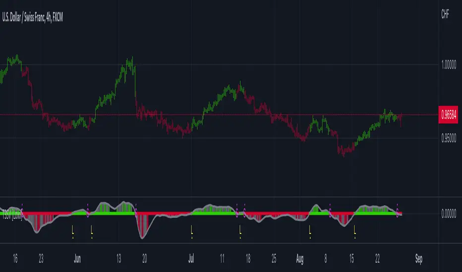
Multi T3 Slopes [Loxx]Multi T3 Slopes is an indicator that checks slopes of 5 (different period) T3 Moving Averages and adds them up to show overall trend. To us this, check for color changes from red to green where there is no red if green is larger than red and there is no red when red is larger than green. When red and green both show up, its a sign of chop.
What is the T3 moving average?
Better Moving Averages Tim Tillson
November 1, 1998
Tim Tillson is a software project manager at Hewlett-Packard, with degrees in Mathematics and Computer Science. He has privately traded options and equities for 15 years.
Introduction
"Digital filtering includes the process of smoothing, predicting, differentiating, integrating, separation of signals, and removal of noise from a signal. Thus many people who do such things are actually using digital filters without realizing that they are; being unacquainted with the theory, they neither understand what they have done nor the possibilities of what they might have done."
This quote from R. W. Hamming applies to the vast majority of indicators in technical analysis . Moving averages, be they simple, weighted, or exponential, are lowpass filters; low frequency components in the signal pass through with little attenuation, while high frequencies are severely reduced.
"Oscillator" type indicators (such as MACD , Momentum, Relative Strength Index ) are another type of digital filter called a differentiator.
Tushar Chande has observed that many popular oscillators are highly correlated, which is sensible because they are trying to measure the rate of change of the underlying time series, i.e., are trying to be the first and second derivatives we all learned about in Calculus.
We use moving averages (lowpass filters) in technical analysis to remove the random noise from a time series, to discern the underlying trend or to determine prices at which we will take action. A perfect moving average would have two attributes:
It would be smooth, not sensitive to random noise in the underlying time series. Another way of saying this is that its derivative would not spuriously alternate between positive and negative values.
It would not lag behind the time series it is computed from. Lag, of course, produces late buy or sell signals that kill profits.
The only way one can compute a perfect moving average is to have knowledge of the future, and if we had that, we would buy one lottery ticket a week rather than trade!
Having said this, we can still improve on the conventional simple, weighted, or exponential moving averages. Here's how:
Two Interesting Moving Averages
We will examine two benchmark moving averages based on Linear Regression analysis.
In both cases, a Linear Regression line of length n is fitted to price data.
I call the first moving average ILRS, which stands for Integral of Linear Regression Slope. One simply integrates the slope of a linear regression line as it is successively fitted in a moving window of length n across the data, with the constant of integration being a simple moving average of the first n points. Put another way, the derivative of ILRS is the linear regression slope. Note that ILRS is not the same as a SMA ( simple moving average ) of length n, which is actually the midpoint of the linear regression line as it moves across the data.
We can measure the lag of moving averages with respect to a linear trend by computing how they behave when the input is a line with unit slope. Both SMA (n) and ILRS(n) have lag of n/2, but ILRS is much smoother than SMA .
Our second benchmark moving average is well known, called EPMA or End Point Moving Average. It is the endpoint of the linear regression line of length n as it is fitted across the data. EPMA hugs the data more closely than a simple or exponential moving average of the same length. The price we pay for this is that it is much noisier (less smooth) than ILRS, and it also has the annoying property that it overshoots the data when linear trends are present.
However, EPMA has a lag of 0 with respect to linear input! This makes sense because a linear regression line will fit linear input perfectly, and the endpoint of the LR line will be on the input line.
These two moving averages frame the tradeoffs that we are facing. On one extreme we have ILRS, which is very smooth and has considerable phase lag. EPMA has 0 phase lag, but is too noisy and overshoots. We would like to construct a better moving average which is as smooth as ILRS, but runs closer to where EPMA lies, without the overshoot.
A easy way to attempt this is to split the difference, i.e. use (ILRS(n)+EPMA(n))/2. This will give us a moving average (call it IE /2) which runs in between the two, has phase lag of n/4 but still inherits considerable noise from EPMA. IE /2 is inspirational, however. Can we build something that is comparable, but smoother? Figure 1 shows ILRS, EPMA, and IE /2.
Filter Techniques
Any thoughtful student of filter theory (or resolute experimenter) will have noticed that you can improve the smoothness of a filter by running it through itself multiple times, at the cost of increasing phase lag.
There is a complementary technique (called twicing by J.W. Tukey) which can be used to improve phase lag. If L stands for the operation of running data through a low pass filter, then twicing can be described by:
L' = L(time series) + L(time series - L(time series))
That is, we add a moving average of the difference between the input and the moving average to the moving average. This is algebraically equivalent to:
2L-L(L)
This is the Double Exponential Moving Average or DEMA , popularized by Patrick Mulloy in TASAC (January/February 1994).
In our taxonomy, DEMA has some phase lag (although it exponentially approaches 0) and is somewhat noisy, comparable to IE /2 indicator.
We will use these two techniques to construct our better moving average, after we explore the first one a little more closely.
Fixing Overshoot
An n-day EMA has smoothing constant alpha=2/(n+1) and a lag of (n-1)/2.
Thus EMA (3) has lag 1, and EMA (11) has lag 5. Figure 2 shows that, if I am willing to incur 5 days of lag, I get a smoother moving average if I run EMA (3) through itself 5 times than if I just take EMA (11) once.
This suggests that if EPMA and DEMA have 0 or low lag, why not run fast versions (eg DEMA (3)) through themselves many times to achieve a smooth result? The problem is that multiple runs though these filters increase their tendency to overshoot the data, giving an unusable result. This is because the amplitude response of DEMA and EPMA is greater than 1 at certain frequencies, giving a gain of much greater than 1 at these frequencies when run though themselves multiple times. Figure 3 shows DEMA (7) and EPMA(7) run through themselves 3 times. DEMA^3 has serious overshoot, and EPMA^3 is terrible.
The solution to the overshoot problem is to recall what we are doing with twicing:
DEMA (n) = EMA (n) + EMA (time series - EMA (n))
The second term is adding, in effect, a smooth version of the derivative to the EMA to achieve DEMA . The derivative term determines how hot the moving average's response to linear trends will be. We need to simply turn down the volume to achieve our basic building block:
EMA (n) + EMA (time series - EMA (n))*.7;
This is algebraically the same as:
EMA (n)*1.7-EMA( EMA (n))*.7;
I have chosen .7 as my volume factor, but the general formula (which I call "Generalized Dema") is:
GD (n,v) = EMA (n)*(1+v)-EMA( EMA (n))*v,
Where v ranges between 0 and 1. When v=0, GD is just an EMA , and when v=1, GD is DEMA . In between, GD is a cooler DEMA . By using a value for v less than 1 (I like .7), we cure the multiple DEMA overshoot problem, at the cost of accepting some additional phase delay. Now we can run GD through itself multiple times to define a new, smoother moving average T3 that does not overshoot the data:
T3(n) = GD ( GD ( GD (n)))
In filter theory parlance, T3 is a six-pole non-linear Kalman filter. Kalman filters are ones which use the error (in this case (time series - EMA (n)) to correct themselves. In Technical Analysis , these are called Adaptive Moving Averages; they track the time series more aggressively when it is making large moves.
Included
Signals: long, short, continuation long, continuation short.
Alerts
Bar coloring
Loxx's expanded source types
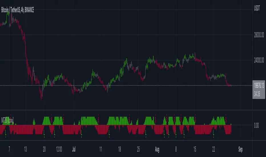
T3 Volatility Quality Index (VQI) w/ DSL & Pips Filtering [Loxx]T3 Volatility Quality Index (VQI) w/ DSL & Pips Filtering is a VQI indicator that uses T3 smoothing and discontinued signal lines to determine breakouts and breakdowns. This also allows filtering by pips.***
What is the Volatility Quality Index ( VQI )?
The idea behind the volatility quality index is to point out the difference between bad and good volatility in order to identify better trade opportunities in the market. This forex indicator works using the True Range algorithm in combination with the open, close, high and low prices.
What are DSL Discontinued Signal Line?
A lot of indicators are using signal lines in order to determine the trend (or some desired state of the indicator) easier. The idea of the signal line is easy : comparing the value to it's smoothed (slightly lagging) state, the idea of current momentum/state is made.
Discontinued signal line is inheriting that simple signal line idea and it is extending it : instead of having one signal line, more lines depending on the current value of the indicator.
"Signal" line is calculated the following way :
When a certain level is crossed into the desired direction, the EMA of that value is calculated for the desired signal line
When that level is crossed into the opposite direction, the previous "signal" line value is simply "inherited" and it becomes a kind of a level
This way it becomes a combination of signal lines and levels that are trying to combine both the good from both methods.
In simple terms, DSL uses the concept of a signal line and betters it by inheriting the previous signal line's value & makes it a level.
What is the T3 moving average?
Better Moving Averages Tim Tillson
November 1, 1998
Tim Tillson is a software project manager at Hewlett-Packard, with degrees in Mathematics and Computer Science. He has privately traded options and equities for 15 years.
Introduction
"Digital filtering includes the process of smoothing, predicting, differentiating, integrating, separation of signals, and removal of noise from a signal. Thus many people who do such things are actually using digital filters without realizing that they are; being unacquainted with the theory, they neither understand what they have done nor the possibilities of what they might have done."
This quote from R. W. Hamming applies to the vast majority of indicators in technical analysis . Moving averages, be they simple, weighted, or exponential, are lowpass filters; low frequency components in the signal pass through with little attenuation, while high frequencies are severely reduced.
"Oscillator" type indicators (such as MACD , Momentum, Relative Strength Index ) are another type of digital filter called a differentiator.
Tushar Chande has observed that many popular oscillators are highly correlated, which is sensible because they are trying to measure the rate of change of the underlying time series, i.e., are trying to be the first and second derivatives we all learned about in Calculus.
We use moving averages (lowpass filters) in technical analysis to remove the random noise from a time series, to discern the underlying trend or to determine prices at which we will take action. A perfect moving average would have two attributes:
It would be smooth, not sensitive to random noise in the underlying time series. Another way of saying this is that its derivative would not spuriously alternate between positive and negative values.
It would not lag behind the time series it is computed from. Lag, of course, produces late buy or sell signals that kill profits.
The only way one can compute a perfect moving average is to have knowledge of the future, and if we had that, we would buy one lottery ticket a week rather than trade!
Having said this, we can still improve on the conventional simple, weighted, or exponential moving averages. Here's how:
Two Interesting Moving Averages
We will examine two benchmark moving averages based on Linear Regression analysis.
In both cases, a Linear Regression line of length n is fitted to price data.
I call the first moving average ILRS, which stands for Integral of Linear Regression Slope. One simply integrates the slope of a linear regression line as it is successively fitted in a moving window of length n across the data, with the constant of integration being a simple moving average of the first n points. Put another way, the derivative of ILRS is the linear regression slope. Note that ILRS is not the same as a SMA ( simple moving average ) of length n, which is actually the midpoint of the linear regression line as it moves across the data.
We can measure the lag of moving averages with respect to a linear trend by computing how they behave when the input is a line with unit slope. Both SMA (n) and ILRS(n) have lag of n/2, but ILRS is much smoother than SMA .
Our second benchmark moving average is well known, called EPMA or End Point Moving Average. It is the endpoint of the linear regression line of length n as it is fitted across the data. EPMA hugs the data more closely than a simple or exponential moving average of the same length. The price we pay for this is that it is much noisier (less smooth) than ILRS, and it also has the annoying property that it overshoots the data when linear trends are present.
However, EPMA has a lag of 0 with respect to linear input! This makes sense because a linear regression line will fit linear input perfectly, and the endpoint of the LR line will be on the input line.
These two moving averages frame the tradeoffs that we are facing. On one extreme we have ILRS, which is very smooth and has considerable phase lag. EPMA has 0 phase lag, but is too noisy and overshoots. We would like to construct a better moving average which is as smooth as ILRS, but runs closer to where EPMA lies, without the overshoot.
A easy way to attempt this is to split the difference, i.e. use (ILRS(n)+EPMA(n))/2. This will give us a moving average (call it IE /2) which runs in between the two, has phase lag of n/4 but still inherits considerable noise from EPMA. IE /2 is inspirational, however. Can we build something that is comparable, but smoother? Figure 1 shows ILRS, EPMA, and IE /2.
Filter Techniques
Any thoughtful student of filter theory (or resolute experimenter) will have noticed that you can improve the smoothness of a filter by running it through itself multiple times, at the cost of increasing phase lag.
There is a complementary technique (called twicing by J.W. Tukey) which can be used to improve phase lag. If L stands for the operation of running data through a low pass filter, then twicing can be described by:
L' = L(time series) + L(time series - L(time series))
That is, we add a moving average of the difference between the input and the moving average to the moving average. This is algebraically equivalent to:
2L-L(L)
This is the Double Exponential Moving Average or DEMA , popularized by Patrick Mulloy in TASAC (January/February 1994).
In our taxonomy, DEMA has some phase lag (although it exponentially approaches 0) and is somewhat noisy, comparable to IE /2 indicator.
We will use these two techniques to construct our better moving average, after we explore the first one a little more closely.
Fixing Overshoot
An n-day EMA has smoothing constant alpha=2/(n+1) and a lag of (n-1)/2.
Thus EMA (3) has lag 1, and EMA (11) has lag 5. Figure 2 shows that, if I am willing to incur 5 days of lag, I get a smoother moving average if I run EMA (3) through itself 5 times than if I just take EMA (11) once.
This suggests that if EPMA and DEMA have 0 or low lag, why not run fast versions (eg DEMA (3)) through themselves many times to achieve a smooth result? The problem is that multiple runs though these filters increase their tendency to overshoot the data, giving an unusable result. This is because the amplitude response of DEMA and EPMA is greater than 1 at certain frequencies, giving a gain of much greater than 1 at these frequencies when run though themselves multiple times. Figure 3 shows DEMA (7) and EPMA(7) run through themselves 3 times. DEMA^3 has serious overshoot, and EPMA^3 is terrible.
The solution to the overshoot problem is to recall what we are doing with twicing:
DEMA (n) = EMA (n) + EMA (time series - EMA (n))
The second term is adding, in effect, a smooth version of the derivative to the EMA to achieve DEMA . The derivative term determines how hot the moving average's response to linear trends will be. We need to simply turn down the volume to achieve our basic building block:
EMA (n) + EMA (time series - EMA (n))*.7;
This is algebraically the same as:
EMA (n)*1.7-EMA( EMA (n))*.7;
I have chosen .7 as my volume factor, but the general formula (which I call "Generalized Dema") is:
GD (n,v) = EMA (n)*(1+v)-EMA( EMA (n))*v,
Where v ranges between 0 and 1. When v=0, GD is just an EMA , and when v=1, GD is DEMA . In between, GD is a cooler DEMA . By using a value for v less than 1 (I like .7), we cure the multiple DEMA overshoot problem, at the cost of accepting some additional phase delay. Now we can run GD through itself multiple times to define a new, smoother moving average T3 that does not overshoot the data:
T3(n) = GD ( GD ( GD (n)))
In filter theory parlance, T3 is a six-pole non-linear Kalman filter. Kalman filters are ones which use the error (in this case (time series - EMA (n)) to correct themselves. In Technical Analysis , these are called Adaptive Moving Averages; they track the time series more aggressively when it is making large moves.
Included
Signals
Alerts
Related indicators
Zero-line Volatility Quality Index (VQI)
Volatility Quality Index w/ Pips Filtering
Variety Moving Average Waddah Attar Explosion (WAE)
***This indicator is tuned to Forex. If you want to make it useful for other tickers, you must change the pip filtering value to match the asset. This means that for BTC, for example, you likely need to use a value of 10,000 or more for pips filter.

T3 PPO [Loxx]T3 PPO is a percentage price oscillator indicator using T3 moving average. This indicator is used to spot reversals. Dark red is upward price exhaustion, dark green is downward price exhaustion.
What is Percentage Price Oscillator (PPO)?
The percentage price oscillator (PPO) is a technical momentum indicator that shows the relationship between two moving averages in percentage terms. The moving averages are a 26-period and 12-period exponential moving average (EMA).
The PPO is used to compare asset performance and volatility, spot divergence that could lead to price reversals, generate trade signals, and help confirm trend direction.
What is the T3 moving average?
Better Moving Averages Tim Tillson
November 1, 1998
Tim Tillson is a software project manager at Hewlett-Packard, with degrees in Mathematics and Computer Science. He has privately traded options and equities for 15 years.
Introduction
"Digital filtering includes the process of smoothing, predicting, differentiating, integrating, separation of signals, and removal of noise from a signal. Thus many people who do such things are actually using digital filters without realizing that they are; being unacquainted with the theory, they neither understand what they have done nor the possibilities of what they might have done."
This quote from R. W. Hamming applies to the vast majority of indicators in technical analysis . Moving averages, be they simple, weighted, or exponential, are lowpass filters; low frequency components in the signal pass through with little attenuation, while high frequencies are severely reduced.
"Oscillator" type indicators (such as MACD , Momentum, Relative Strength Index ) are another type of digital filter called a differentiator.
Tushar Chande has observed that many popular oscillators are highly correlated, which is sensible because they are trying to measure the rate of change of the underlying time series, i.e., are trying to be the first and second derivatives we all learned about in Calculus.
We use moving averages (lowpass filters) in technical analysis to remove the random noise from a time series, to discern the underlying trend or to determine prices at which we will take action. A perfect moving average would have two attributes:
It would be smooth, not sensitive to random noise in the underlying time series. Another way of saying this is that its derivative would not spuriously alternate between positive and negative values.
It would not lag behind the time series it is computed from. Lag, of course, produces late buy or sell signals that kill profits.
The only way one can compute a perfect moving average is to have knowledge of the future, and if we had that, we would buy one lottery ticket a week rather than trade!
Having said this, we can still improve on the conventional simple, weighted, or exponential moving averages. Here's how:
Two Interesting Moving Averages
We will examine two benchmark moving averages based on Linear Regression analysis.
In both cases, a Linear Regression line of length n is fitted to price data.
I call the first moving average ILRS, which stands for Integral of Linear Regression Slope. One simply integrates the slope of a linear regression line as it is successively fitted in a moving window of length n across the data, with the constant of integration being a simple moving average of the first n points. Put another way, the derivative of ILRS is the linear regression slope. Note that ILRS is not the same as a SMA ( simple moving average ) of length n, which is actually the midpoint of the linear regression line as it moves across the data.
We can measure the lag of moving averages with respect to a linear trend by computing how they behave when the input is a line with unit slope. Both SMA (n) and ILRS(n) have lag of n/2, but ILRS is much smoother than SMA .
Our second benchmark moving average is well known, called EPMA or End Point Moving Average. It is the endpoint of the linear regression line of length n as it is fitted across the data. EPMA hugs the data more closely than a simple or exponential moving average of the same length. The price we pay for this is that it is much noisier (less smooth) than ILRS, and it also has the annoying property that it overshoots the data when linear trends are present.
However, EPMA has a lag of 0 with respect to linear input! This makes sense because a linear regression line will fit linear input perfectly, and the endpoint of the LR line will be on the input line.
These two moving averages frame the tradeoffs that we are facing. On one extreme we have ILRS, which is very smooth and has considerable phase lag. EPMA has 0 phase lag, but is too noisy and overshoots. We would like to construct a better moving average which is as smooth as ILRS, but runs closer to where EPMA lies, without the overshoot.
A easy way to attempt this is to split the difference, i.e. use (ILRS(n)+EPMA(n))/2. This will give us a moving average (call it IE /2) which runs in between the two, has phase lag of n/4 but still inherits considerable noise from EPMA. IE /2 is inspirational, however. Can we build something that is comparable, but smoother? Figure 1 shows ILRS, EPMA, and IE /2.
Filter Techniques
Any thoughtful student of filter theory (or resolute experimenter) will have noticed that you can improve the smoothness of a filter by running it through itself multiple times, at the cost of increasing phase lag.
There is a complementary technique (called twicing by J.W. Tukey) which can be used to improve phase lag. If L stands for the operation of running data through a low pass filter, then twicing can be described by:
L' = L(time series) + L(time series - L(time series))
That is, we add a moving average of the difference between the input and the moving average to the moving average. This is algebraically equivalent to:
2L-L(L)
This is the Double Exponential Moving Average or DEMA , popularized by Patrick Mulloy in TASAC (January/February 1994).
In our taxonomy, DEMA has some phase lag (although it exponentially approaches 0) and is somewhat noisy, comparable to IE /2 indicator.
We will use these two techniques to construct our better moving average, after we explore the first one a little more closely.
Fixing Overshoot
An n-day EMA has smoothing constant alpha=2/(n+1) and a lag of (n-1)/2.
Thus EMA (3) has lag 1, and EMA (11) has lag 5. Figure 2 shows that, if I am willing to incur 5 days of lag, I get a smoother moving average if I run EMA (3) through itself 5 times than if I just take EMA (11) once.
This suggests that if EPMA and DEMA have 0 or low lag, why not run fast versions (eg DEMA (3)) through themselves many times to achieve a smooth result? The problem is that multiple runs though these filters increase their tendency to overshoot the data, giving an unusable result. This is because the amplitude response of DEMA and EPMA is greater than 1 at certain frequencies, giving a gain of much greater than 1 at these frequencies when run though themselves multiple times. Figure 3 shows DEMA (7) and EPMA(7) run through themselves 3 times. DEMA^3 has serious overshoot, and EPMA^3 is terrible.
The solution to the overshoot problem is to recall what we are doing with twicing:
DEMA (n) = EMA (n) + EMA (time series - EMA (n))
The second term is adding, in effect, a smooth version of the derivative to the EMA to achieve DEMA . The derivative term determines how hot the moving average's response to linear trends will be. We need to simply turn down the volume to achieve our basic building block:
EMA (n) + EMA (time series - EMA (n))*.7;
This is algebraically the same as:
EMA (n)*1.7-EMA( EMA (n))*.7;
I have chosen .7 as my volume factor, but the general formula (which I call "Generalized Dema") is:
GD (n,v) = EMA (n)*(1+v)-EMA( EMA (n))*v,
Where v ranges between 0 and 1. When v=0, GD is just an EMA , and when v=1, GD is DEMA . In between, GD is a cooler DEMA . By using a value for v less than 1 (I like .7), we cure the multiple DEMA overshoot problem, at the cost of accepting some additional phase delay. Now we can run GD through itself multiple times to define a new, smoother moving average T3 that does not overshoot the data:
T3(n) = GD ( GD ( GD (n)))
In filter theory parlance, T3 is a six-pole non-linear Kalman filter. Kalman filters are ones which use the error (in this case (time series - EMA (n)) to correct themselves. In Technical Analysis , these are called Adaptive Moving Averages; they track the time series more aggressively when it is making large moves.
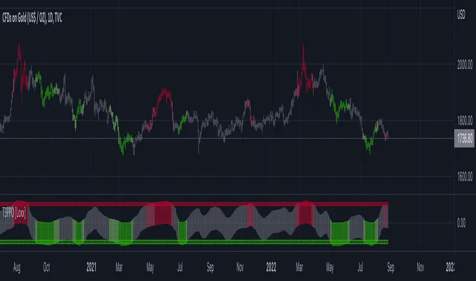
VHF-Adaptive T3 iTrend [Loxx]VHF-Adaptive T3 iTrend is an iTrend indicator with T3 smoothing and Vertical Horizontal Filter Adaptive period input. iTrend is used to determine where the trend starts and ends. You'll notice that the noise filter on this one is extreme. Adjust the period inputs accordingly to suit your take and your backtest requirements. This is also useful for scalping lower timeframes. Enjoy!
What is VHF Adaptive Period?
Vertical Horizontal Filter (VHF) was created by Adam White to identify trending and ranging markets. VHF measures the level of trend activity, similar to ADX DI. Vertical Horizontal Filter does not, itself, generate trading signals, but determines whether signals are taken from trend or momentum indicators. Using this trend information, one is then able to derive an average cycle length.
What is the T3 moving average?
Better Moving Averages Tim Tillson
November 1, 1998
Tim Tillson is a software project manager at Hewlett-Packard, with degrees in Mathematics and Computer Science. He has privately traded options and equities for 15 years.
Introduction
"Digital filtering includes the process of smoothing, predicting, differentiating, integrating, separation of signals, and removal of noise from a signal. Thus many people who do such things are actually using digital filters without realizing that they are; being unacquainted with the theory, they neither understand what they have done nor the possibilities of what they might have done."
This quote from R. W. Hamming applies to the vast majority of indicators in technical analysis . Moving averages, be they simple, weighted, or exponential, are lowpass filters; low frequency components in the signal pass through with little attenuation, while high frequencies are severely reduced.
"Oscillator" type indicators (such as MACD , Momentum, Relative Strength Index ) are another type of digital filter called a differentiator.
Tushar Chande has observed that many popular oscillators are highly correlated, which is sensible because they are trying to measure the rate of change of the underlying time series, i.e., are trying to be the first and second derivatives we all learned about in Calculus.
We use moving averages (lowpass filters) in technical analysis to remove the random noise from a time series, to discern the underlying trend or to determine prices at which we will take action. A perfect moving average would have two attributes:
It would be smooth, not sensitive to random noise in the underlying time series. Another way of saying this is that its derivative would not spuriously alternate between positive and negative values.
It would not lag behind the time series it is computed from. Lag, of course, produces late buy or sell signals that kill profits.
The only way one can compute a perfect moving average is to have knowledge of the future, and if we had that, we would buy one lottery ticket a week rather than trade!
Having said this, we can still improve on the conventional simple, weighted, or exponential moving averages. Here's how:
Two Interesting Moving Averages
We will examine two benchmark moving averages based on Linear Regression analysis.
In both cases, a Linear Regression line of length n is fitted to price data.
I call the first moving average ILRS, which stands for Integral of Linear Regression Slope. One simply integrates the slope of a linear regression line as it is successively fitted in a moving window of length n across the data, with the constant of integration being a simple moving average of the first n points. Put another way, the derivative of ILRS is the linear regression slope. Note that ILRS is not the same as a SMA ( simple moving average ) of length n, which is actually the midpoint of the linear regression line as it moves across the data.
We can measure the lag of moving averages with respect to a linear trend by computing how they behave when the input is a line with unit slope. Both SMA (n) and ILRS(n) have lag of n/2, but ILRS is much smoother than SMA .
Our second benchmark moving average is well known, called EPMA or End Point Moving Average. It is the endpoint of the linear regression line of length n as it is fitted across the data. EPMA hugs the data more closely than a simple or exponential moving average of the same length. The price we pay for this is that it is much noisier (less smooth) than ILRS, and it also has the annoying property that it overshoots the data when linear trends are present.
However, EPMA has a lag of 0 with respect to linear input! This makes sense because a linear regression line will fit linear input perfectly, and the endpoint of the LR line will be on the input line.
These two moving averages frame the tradeoffs that we are facing. On one extreme we have ILRS, which is very smooth and has considerable phase lag. EPMA has 0 phase lag, but is too noisy and overshoots. We would like to construct a better moving average which is as smooth as ILRS, but runs closer to where EPMA lies, without the overshoot.
A easy way to attempt this is to split the difference, i.e. use (ILRS(n)+EPMA(n))/2. This will give us a moving average (call it IE /2) which runs in between the two, has phase lag of n/4 but still inherits considerable noise from EPMA. IE /2 is inspirational, however. Can we build something that is comparable, but smoother? Figure 1 shows ILRS, EPMA, and IE /2.
Filter Techniques
Any thoughtful student of filter theory (or resolute experimenter) will have noticed that you can improve the smoothness of a filter by running it through itself multiple times, at the cost of increasing phase lag.
There is a complementary technique (called twicing by J.W. Tukey) which can be used to improve phase lag. If L stands for the operation of running data through a low pass filter, then twicing can be described by:
L' = L(time series) + L(time series - L(time series))
That is, we add a moving average of the difference between the input and the moving average to the moving average. This is algebraically equivalent to:
2L-L(L)
This is the Double Exponential Moving Average or DEMA , popularized by Patrick Mulloy in TASAC (January/February 1994).
In our taxonomy, DEMA has some phase lag (although it exponentially approaches 0) and is somewhat noisy, comparable to IE /2 indicator.
We will use these two techniques to construct our better moving average, after we explore the first one a little more closely.
Fixing Overshoot
An n-day EMA has smoothing constant alpha=2/(n+1) and a lag of (n-1)/2.
Thus EMA (3) has lag 1, and EMA (11) has lag 5. Figure 2 shows that, if I am willing to incur 5 days of lag, I get a smoother moving average if I run EMA (3) through itself 5 times than if I just take EMA (11) once.
This suggests that if EPMA and DEMA have 0 or low lag, why not run fast versions (eg DEMA (3)) through themselves many times to achieve a smooth result? The problem is that multiple runs though these filters increase their tendency to overshoot the data, giving an unusable result. This is because the amplitude response of DEMA and EPMA is greater than 1 at certain frequencies, giving a gain of much greater than 1 at these frequencies when run though themselves multiple times. Figure 3 shows DEMA (7) and EPMA(7) run through themselves 3 times. DEMA^3 has serious overshoot, and EPMA^3 is terrible.
The solution to the overshoot problem is to recall what we are doing with twicing:
DEMA (n) = EMA (n) + EMA (time series - EMA (n))
The second term is adding, in effect, a smooth version of the derivative to the EMA to achieve DEMA . The derivative term determines how hot the moving average's response to linear trends will be. We need to simply turn down the volume to achieve our basic building block:
EMA (n) + EMA (time series - EMA (n))*.7;
This is algebraically the same as:
EMA (n)*1.7-EMA( EMA (n))*.7;
I have chosen .7 as my volume factor, but the general formula (which I call "Generalized Dema") is:
GD (n,v) = EMA (n)*(1+v)-EMA( EMA (n))*v,
Where v ranges between 0 and 1. When v=0, GD is just an EMA , and when v=1, GD is DEMA . In between, GD is a cooler DEMA . By using a value for v less than 1 (I like .7), we cure the multiple DEMA overshoot problem, at the cost of accepting some additional phase delay. Now we can run GD through itself multiple times to define a new, smoother moving average T3 that does not overshoot the data:
T3(n) = GD ( GD ( GD (n)))
In filter theory parlance, T3 is a six-pole non-linear Kalman filter. Kalman filters are ones which use the error (in this case (time series - EMA (n)) to correct themselves. In Technical Analysis , these are called Adaptive Moving Averages; they track the time series more aggressively when it is making large moves.
Included
Bar coloring
Alerts
Signals
Loxx's Expanded Source Types
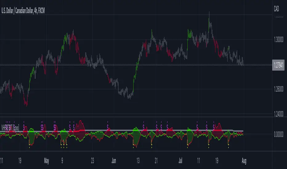
CFB-Adaptive CCI w/ T3 Smoothing [Loxx]CFB-Adaptive CCI w/ T3 Smoothing is a CCI indicator with adaptive period inputs and T3 smoothing. Jurik's Composite Fractal Behavior is used to created dynamic period input.
What is Composite Fractal Behavior ( CFB )?
All around you mechanisms adjust themselves to their environment. From simple thermostats that react to air temperature to computer chips in modern cars that respond to changes in engine temperature, r.p.m.'s, torque, and throttle position. It was only a matter of time before fast desktop computers applied the mathematics of self-adjustment to systems that trade the financial markets.
Unlike basic systems with fixed formulas, an adaptive system adjusts its own equations. For example, start with a basic channel breakout system that uses the highest closing price of the last N bars as a threshold for detecting breakouts on the up side. An adaptive and improved version of this system would adjust N according to market conditions, such as momentum, price volatility or acceleration.
Since many systems are based directly or indirectly on cycles, another useful measure of market condition is the periodic length of a price chart's dominant cycle, (DC), that cycle with the greatest influence on price action.
The utility of this new DC measure was noted by author Murray Ruggiero in the January '96 issue of Futures Magazine. In it. Mr. Ruggiero used it to adaptive adjust the value of N in a channel breakout system. He then simulated trading 15 years of D-Mark futures in order to compare its performance to a similar system that had a fixed optimal value of N. The adaptive version produced 20% more profit!
This DC index utilized the popular MESA algorithm (a formulation by John Ehlers adapted from Burg's maximum entropy algorithm, MEM). Unfortunately, the DC approach is problematic when the market has no real dominant cycle momentum, because the mathematics will produce a value whether or not one actually exists! Therefore, we developed a proprietary indicator that does not presuppose the presence of market cycles. It's called CFB (Composite Fractal Behavior) and it works well whether or not the market is cyclic.
CFB examines price action for a particular fractal pattern, categorizes them by size, and then outputs a composite fractal size index. This index is smooth, timely and accurate
Essentially, CFB reveals the length of the market's trending action time frame. Long trending activity produces a large CFB index and short choppy action produces a small index value. Investors have found many applications for CFB which involve scaling other existing technical indicators adaptively, on a bar-to-bar basis.
What is Jurik Volty used in the Juirk Filter?
One of the lesser known qualities of Juirk smoothing is that the Jurik smoothing process is adaptive. "Jurik Volty" (a sort of market volatility ) is what makes Jurik smoothing adaptive. The Jurik Volty calculation can be used as both a standalone indicator and to smooth other indicators that you wish to make adaptive.
What is the Jurik Moving Average?
Have you noticed how moving averages add some lag (delay) to your signals? ... especially when price gaps up or down in a big move, and you are waiting for your moving average to catch up? Wait no more! JMA eliminates this problem forever and gives you the best of both worlds: low lag and smooth lines.
Ideally, you would like a filtered signal to be both smooth and lag-free. Lag causes delays in your trades, and increasing lag in your indicators typically result in lower profits. In other words, late comers get what's left on the table after the feast has already begun.
What is the T3 moving average?
Better Moving Averages Tim Tillson
November 1, 1998
Tim Tillson is a software project manager at Hewlett-Packard, with degrees in Mathematics and Computer Science. He has privately traded options and equities for 15 years.
Introduction
"Digital filtering includes the process of smoothing, predicting, differentiating, integrating, separation of signals, and removal of noise from a signal. Thus many people who do such things are actually using digital filters without realizing that they are; being unacquainted with the theory, they neither understand what they have done nor the possibilities of what they might have done."
This quote from R. W. Hamming applies to the vast majority of indicators in technical analysis . Moving averages, be they simple, weighted, or exponential, are lowpass filters; low frequency components in the signal pass through with little attenuation, while high frequencies are severely reduced.
"Oscillator" type indicators (such as MACD , Momentum, Relative Strength Index ) are another type of digital filter called a differentiator.
Tushar Chande has observed that many popular oscillators are highly correlated, which is sensible because they are trying to measure the rate of change of the underlying time series, i.e., are trying to be the first and second derivatives we all learned about in Calculus.
We use moving averages (lowpass filters) in technical analysis to remove the random noise from a time series, to discern the underlying trend or to determine prices at which we will take action. A perfect moving average would have two attributes:
It would be smooth, not sensitive to random noise in the underlying time series. Another way of saying this is that its derivative would not spuriously alternate between positive and negative values.
It would not lag behind the time series it is computed from. Lag, of course, produces late buy or sell signals that kill profits.
The only way one can compute a perfect moving average is to have knowledge of the future, and if we had that, we would buy one lottery ticket a week rather than trade!
Having said this, we can still improve on the conventional simple, weighted, or exponential moving averages. Here's how:
Two Interesting Moving Averages
We will examine two benchmark moving averages based on Linear Regression analysis.
In both cases, a Linear Regression line of length n is fitted to price data.
I call the first moving average ILRS, which stands for Integral of Linear Regression Slope. One simply integrates the slope of a linear regression line as it is successively fitted in a moving window of length n across the data, with the constant of integration being a simple moving average of the first n points. Put another way, the derivative of ILRS is the linear regression slope. Note that ILRS is not the same as a SMA ( simple moving average ) of length n, which is actually the midpoint of the linear regression line as it moves across the data.
We can measure the lag of moving averages with respect to a linear trend by computing how they behave when the input is a line with unit slope. Both SMA (n) and ILRS(n) have lag of n/2, but ILRS is much smoother than SMA .
Our second benchmark moving average is well known, called EPMA or End Point Moving Average. It is the endpoint of the linear regression line of length n as it is fitted across the data. EPMA hugs the data more closely than a simple or exponential moving average of the same length. The price we pay for this is that it is much noisier (less smooth) than ILRS, and it also has the annoying property that it overshoots the data when linear trends are present.
However, EPMA has a lag of 0 with respect to linear input! This makes sense because a linear regression line will fit linear input perfectly, and the endpoint of the LR line will be on the input line.
These two moving averages frame the tradeoffs that we are facing. On one extreme we have ILRS, which is very smooth and has considerable phase lag. EPMA has 0 phase lag, but is too noisy and overshoots. We would like to construct a better moving average which is as smooth as ILRS, but runs closer to where EPMA lies, without the overshoot.
A easy way to attempt this is to split the difference, i.e. use (ILRS(n)+EPMA(n))/2. This will give us a moving average (call it IE /2) which runs in between the two, has phase lag of n/4 but still inherits considerable noise from EPMA. IE /2 is inspirational, however. Can we build something that is comparable, but smoother? Figure 1 shows ILRS, EPMA, and IE /2.
Filter Techniques
Any thoughtful student of filter theory (or resolute experimenter) will have noticed that you can improve the smoothness of a filter by running it through itself multiple times, at the cost of increasing phase lag.
There is a complementary technique (called twicing by J.W. Tukey) which can be used to improve phase lag. If L stands for the operation of running data through a low pass filter, then twicing can be described by:
L' = L(time series) + L(time series - L(time series))
That is, we add a moving average of the difference between the input and the moving average to the moving average. This is algebraically equivalent to:
2L-L(L)
This is the Double Exponential Moving Average or DEMA , popularized by Patrick Mulloy in TASAC (January/February 1994).
In our taxonomy, DEMA has some phase lag (although it exponentially approaches 0) and is somewhat noisy, comparable to IE /2 indicator.
We will use these two techniques to construct our better moving average, after we explore the first one a little more closely.
Fixing Overshoot
An n-day EMA has smoothing constant alpha=2/(n+1) and a lag of (n-1)/2.
Thus EMA (3) has lag 1, and EMA (11) has lag 5. Figure 2 shows that, if I am willing to incur 5 days of lag, I get a smoother moving average if I run EMA (3) through itself 5 times than if I just take EMA (11) once.
This suggests that if EPMA and DEMA have 0 or low lag, why not run fast versions (eg DEMA (3)) through themselves many times to achieve a smooth result? The problem is that multiple runs though these filters increase their tendency to overshoot the data, giving an unusable result. This is because the amplitude response of DEMA and EPMA is greater than 1 at certain frequencies, giving a gain of much greater than 1 at these frequencies when run though themselves multiple times. Figure 3 shows DEMA (7) and EPMA(7) run through themselves 3 times. DEMA^3 has serious overshoot, and EPMA^3 is terrible.
The solution to the overshoot problem is to recall what we are doing with twicing:
DEMA (n) = EMA (n) + EMA (time series - EMA (n))
The second term is adding, in effect, a smooth version of the derivative to the EMA to achieve DEMA . The derivative term determines how hot the moving average's response to linear trends will be. We need to simply turn down the volume to achieve our basic building block:
EMA (n) + EMA (time series - EMA (n))*.7;
This is algebraically the same as:
EMA (n)*1.7-EMA( EMA (n))*.7;
I have chosen .7 as my volume factor, but the general formula (which I call "Generalized Dema") is:
GD (n,v) = EMA (n)*(1+v)-EMA( EMA (n))*v,
Where v ranges between 0 and 1. When v=0, GD is just an EMA , and when v=1, GD is DEMA . In between, GD is a cooler DEMA . By using a value for v less than 1 (I like .7), we cure the multiple DEMA overshoot problem, at the cost of accepting some additional phase delay. Now we can run GD through itself multiple times to define a new, smoother moving average T3 that does not overshoot the data:
T3(n) = GD ( GD ( GD (n)))
In filter theory parlance, T3 is a six-pole non-linear Kalman filter. Kalman filters are ones which use the error (in this case (time series - EMA (n)) to correct themselves. In Technical Analysis , these are called Adaptive Moving Averages; they track the time series more aggressively when it is making large moves.
Included:
Bar coloring
Signals
Alerts
