Hazel nut BB Strategy, volume base- lite versionHazel nut BB Strategy, volume base — lite version
Having knowledge and information in financial markets is only useful when a trader operates with a well-defined trading strategy. Trading strategies assist in capital management, profit-taking, and reducing potential losses.
This strategy is built upon the core principle of supply and demand dynamics. Alongside this foundation, one of the widely used technical tools — the Bollinger Bands — is employed to structure a framework for profit management and risk control.
In this strategy, the interaction of these tools is explained in detail. A key point to note is that for calculating buy and sell volumes, a lower timeframe function is used. When applied with a tick-level resolution, this provides the most precise measurement of buyer/seller flows. However, this comes with a limitation of reduced historical depth. Users should be aware of this trade-off: if precise tick-level data is required, shorter timeframes should be considered to extend historical coverage .
The strategy offers multiple configuration options. Nevertheless, it should be treated strictly as a supportive tool rather than a standalone trading system. Decisions must integrate personal analysis and other instruments. For example, in highly volatile assets with narrow ranges, it is recommended to adjust profit-taking and stop-loss percentages to smaller values.
◉ Volume Settings
• Buyer and seller volume (up/down volume) are requested from a lower timeframe, with an option to override the automatic resolution.
• A global lookback period is applied to calculate moving averages and cumulative sums of buy/sell/delta volumes.
• Ratios of buyers/sellers to total volume are derived both on the current bar and across the lookback window.
◉ Bollinger Band
• Bands are computed using configurable moving averages (SMA, EMA, RMA, WMA, VWMA).
• Inputs allow control of length, standard deviation multiplier, and offset.
• The basis, upper, and lower bands are plotted, with a shaded background between them.
◉ Progress & Proximity
• Relative position of the price to the Bollinger basis is expressed as percentages (qPlus/qMinus).
• “Near band” conditions are triggered when price progress toward the upper or lower band exceeds a user-defined threshold (%).
• A signed score (sScore) represents how far the close has moved above or below the basis relative to band width.
◉ Info Table
• Optional compact table summarizing:
• - Upper/lower band margins
• - Buyer/seller volumes with moving averages
• - Delta and cumulative delta
• - Buyer/seller ratios per bar and across the window
• - Money flow values (buy/sell/delta × price) for bar-level and summed periods
• The table is neutral-colored and resizable for different chart layouts.
◉ Zone Event Gate
• Tracks entry into and exit from “near band” zones.
• Arming logic: a side is armed when price enters a band proximity zone.
• Trigger logic: on exit, a trade event is generated if cumulative buyer or seller volume dominates over a configurable window.
◉ Trading Logic
• Orders are placed only on zone-exit events, conditional on volume dominance.
• Position sizing is defined as a fixed percentage of strategy equity.
• Long entries occur when leaving the lower zone with buyer dominance; short entries occur when leaving the upper zone with seller dominance.
◉ Exit Rules
• Open positions are managed by a strict priority sequence:
• 1. Stop-loss (% of entry price)
• 2. Take-profit (% of entry price)
• 3. Opposite-side event (zone exit with dominance in the other direction)
• Stop-loss and take-profit levels are configurable
◉ Notes
• This lite version is intended to demonstrate the interaction of Bollinger Bands and volume-based dominance logic.
• It provides a framework to observe how price reacts at band boundaries under varying buy/sell pressure, and how zone exits can be systematically converted into entry/exit signals.
When configuring this strategy, it is essential to carefully review the settings within the Strategy Tester. Ensure that the chosen parameters and historical data options are correctly aligned with the intended use. Accurate back testing depends on applying proper configurations for historical reference. The figure below illustrates sample result and configuration type.
Tìm kiếm tập lệnh với "zone"

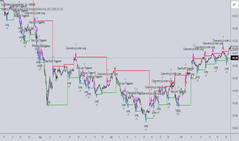
Liquidity + Internal Market Shift StrategyLiquidity + Internal Market Shift Strategy
This strategy combines liquidity zone analysis with the internal market structure, aiming to identify high-probability entry points. It uses key liquidity levels (local highs and lows) to track the price's interaction with significant market levels and then employs internal market shifts to trigger trades.
Key Features:
Internal Shift Logic: Instead of relying on traditional candlestick patterns like engulfing candles, this strategy utilizes internal market shifts. A bullish shift occurs when the price breaks previous bearish levels, and a bearish shift happens when the price breaks previous bullish levels, indicating a change in market direction.
Liquidity Zones: The strategy dynamically identifies key liquidity zones (local highs and lows) to detect potential reversal points and prevent trades in weak market conditions.
Mode Options: You can choose to run the strategy in "Both," "Bullish Only," or "Bearish Only" modes, allowing for flexibility based on market conditions.
Stop-Loss and Take-Profit: Customizable stop-loss and take-profit levels are integrated to manage risk and lock in profits.
Time Range Control: You can specify the time range for trading, ensuring the strategy only operates during the desired period.
This strategy is ideal for traders who want to combine liquidity analysis with internal structure shifts for precise market entries and exits.
This description clearly outlines the strategy's logic, the flexibility it provides, and how it works. You can adjust it further to match your personal trading style or preferences!
JMA Quantum Edge: Adaptive Precision Trading System JMA Quantum Edge: Adaptive Precision Trading System - Enhanced Visuals & Risk Management
Get ready to experience a groundbreaking trading strategy that adapts in real-time to market conditions! This powerful, open-source script combines advanced technical analysis with state-of-the-art risk management tools, designed to give you the edge you need in today's dynamic markets.
What It Does:
Adaptive JMA Indicator:
Utilizes a custom Jurik Moving Average (JMA) that adjusts its sensitivity based on market volatility, ensuring you get precise signals even in the most fluctuating environments.
Dynamic Risk Management:
Features built-in support for partial exits (scaling out) to secure profits, along with an optional Kelly Criterion-based position sizing that tailors your exposure based on historical performance metrics.
Robust Error Handling:
Incorporates market condition filters—like minimum volume and maximum allowed gap percentage—to ensure trades are only executed under favorable conditions.
Vivid Visual Enhancements:
Enjoy an animated background that reflects market momentum, dynamic pivot markers, and clearly drawn trend channels. Plus, interactive tables provide real-time performance analytics and detailed error metrics.
Fully Customizable:
With a comprehensive set of inputs, you can easily tailor the strategy to your personal trading style and market preferences. Adjust everything from JMA parameters to refresh intervals for tables and labels!
How to Use It:
Add the Script:
Copy and paste the script into the Pine Script Editor on TradingView and click “Add to Chart.”
Configure Your Settings:
Customize your risk management (capital, commission, position sizing, partial exits, etc.) and tweak the JMA settings to match your preferred trading style. Use the extensive input panel to adjust visuals, alerts, and more.
Backtest & Optimize:
Run the strategy in the Strategy Tester to analyze its historical performance. Monitor real-time analytics and error metrics via the interactive tables, and fine-tune your parameters for optimal performance.
Go Live with Confidence:
Once you're satisfied with the backtest results, use the generated signals for live trading, and let the system help you stay ahead in fast-paced markets!
How to use the imputs:
This cutting-edge strategy is designed to adapt to changing market conditions and offers you complete control over your trading parameters. Here’s a breakdown of what each group of inputs does and how you should use them:
Risk Management & Trade Settings
Recalculate on Every Tick:
What it does: When enabled, the strategy recalculates on every price update.
Recommendation: Leave it true for fast charts.
Initial Capital:
What it does: Sets your starting capital for backtesting, which influences position sizing and performance metrics.
Recommendation: Start with $10,000 (or adjust according to your trading capital).
Commission (%):
What it does: Simulates the cost per trade.
Recommendation: Use a realistic rate (e.g., 0.04%).
Position Size & Quantity Type:
What they do: Define how large each trade will be. Choose between a fixed unit amount or a percentage of equity.
Recommendation: For beginners, the default fixed value is a good start. Experiment later with percentage-based sizing if needed.
Order Comment:
What it does: Adds a label to your orders for easier tracking.
Allow Reverse Orders:
What it does: If disabled, the strategy will close opposing positions before entering a new trade, reducing conflicts.
Enable Dynamic Position Sizing:
What it does: Adjusts trade size based on current volatility.
Recommendation: Beginners may start with this disabled until they understand basic sizing.
Partial Exit Inputs:
What they do:
Enable Partial Exits: When turned on, you can scale out of your position to lock in profits.
Partial Exit Profit (%): The profit percentage that triggers a partial exit.
Partial Exit Percentage: The percentage of your current position to exit. Recommendation: Use defaults (e.g., 5% profit, 50% exit) to secure profits gradually.
Kelly Criterion Option:
What it does: When enabled, adjusts your position sizing using historical performance (win rate and profit factor).
Recommendation: Beginners might leave this disabled until comfortable with backtest performance metrics.
Market Condition Filters:
What they do:
Minimum Volume: Ensures trades occur only when there’s sufficient market activity.
Maximum Gap (%): Prevents trading if there’s an unusually large gap between the previous close and current open. Recommendation: Defaults work well for most markets. If trades seem erratic, consider tightening these limits.
JMA Settings
Price Source:
What it does: The input series for the JMA calculation, typically set to the closing price.
JMA Length:
What it does: Controls the smoothing period of the JMA. Lower values are more sensitive; higher values smooth out the noise. Recommendation: Start with 21.
JMA Phase & Power:
What they do: Adjust how responsive the JMA is. Phase controls timing; power adjusts the intensity. Recommendation: Default settings (63 phase and 3 power) are a balanced starting point.
Visual Settings & Style
Show JMA Line, Pivot Lines, and Pivot Labels:
What they do: Toggle visual elements on your chart for easier signal identification.
Pivot History Count:
What it does: Limits how many historical pivot markers are displayed.
Color Settings (Up/Down Neon Colors):
What they do: Set the visual cues for buy and sell signals.
Pivot Marker & Line Style:
What they do: Choose the style and thickness of your pivot markers and lines.
Show Stats Panel:
What it does: Displays real-time performance and error metrics.
Dynamic Background & Visual Enhancements
Animate Background:
What it does: Changes the background color based on market momentum.
Show Trend Channels & Volume Zones:
What they do: Draw trend channels and highlight areas of high volatility/volume.
Show Data-Rich Labels:
What it does: Displays key metrics like volume, error percentage, and momentum on the chart.
High Volatility Threshold:
What it does: Determines the multiplier for when the chart background should change due to high volatility.
Multi-Timeframe Settings
Higher Timeframe:
What it does: Uses a higher timeframe’s JMA for trend confirmation. Recommendation: Use Daily ('D') or Weekly ('W') for broader trend analysis.
Show HTF Trend Zone & Opacity:
What they do: Display a visual zone from the higher timeframe to help confirm trends.
6. Trailing Stop Settings
Trailing Stop ATR Factor & Offset Multiplier:
What they do: Calculate trailing stops based on the Average True Range (ATR), adjusting stop distances dynamically. Recommendation: Default settings are a good balance but can be fine-tuned based on asset volatility.
Alerts & Notifications
Alerts on Pivot Formation & JMA Crossover:
What they do: Notify you when key events occur.
Dynamic Power Threshold:
What it does: Sets the sensitivity for dynamic alerts.
8. Static Stop Loss / Take Profit
Static Stop Loss (%) & Take Profit (%):
What they do: Allow you to set fixed stop loss or take profit levels. Recommendation: Leave them at 0 to disable if you prefer dynamic risk management, or set them if you have strict risk/reward preferences.
Advanced Settings
ATR Length:
What it does: Determines the period for ATR calculation, impacting trailing stop sensitivity. Recommendation: Start with 14.
Optimization Feedback & Enhanced Error Analysis
Error Metric Length & Error Threshold (%):
What they do: Calculate error metrics (like average error, skewness, and kurtosis) to help you fine-tune the JMA. Recommendation: Use the defaults and adjust if the error metrics seem off during backtesting.
UI - User-Driven Tweaking & Table Customization
Parameter Tweaker Panel, Debug/Performance Table Settings:
What they do: Provide interactive tables that display real-time performance, error metrics, and allow you to monitor strategy parameters.
Refresh Frequency Options (Table & Label Refresh Intervals):
What they do: Set how often the tables and labels update.
Recommendation: Start with an interval of 1 bar; increase it if your chart is too busy.
Important for Beginners:
Default Settings:
All default values have been chosen for balanced performance across different markets. If you ever experience unexpected behavior, start by resetting the inputs to their defaults.
Step-by-Step Adjustments:
Experiment by changing one setting at a time while observing how the strategy’s signals and performance metrics change. This will help you understand the impact of each parameter.
Resetting to Defaults:
If things seem off or you’re not getting the expected results, you can always reset the indicator. Either reload the script or use the “Reset Inputs” option (if available) to revert to the default settings.
Jump in, experiment, and enjoy the power of adaptive precision trading. This strategy is built to grow with your skills—have fun exploring and refining your trading edge!
Happy trading!

RastaRasta — Educational Strategy (Pine v5)
Momentum · Smoothing · Trend Study
Overview
The Rasta Strategy is a visual and educational framework designed to help traders study momentum transitions using the interaction between a fast-reacting EMA line and a slower smoothed reference line.
It is not a signal generator or profit system; it’s a learning tool for understanding how smoothing, crossovers, and filters interact under different market conditions.
The script displays:
A primary EMA line (the fast reactive wave).
A Smoothed line (using your chosen smoothing method).
Optional fog zones between them for quick visual context.
Optional DNA rungs connecting both lines to illustrate volatility compression and expansion.
Optional EMA 8 / EMA 21 trend filter to observe higher-time-frame alignment.
Core Idea
The Rasta model focuses on wave interaction. When the fast EMA crosses above the smoothed line, it reflects a shift in short-term momentum relative to background trend pressure. Cross-unders suggest weakening or reversal.
Rather than treating this as a trading “signal,” use it to observe structure, study trend alignment, and test how smoothing type affects reaction speed.
Smoothing Types Explained
The script lets you experiment with multiple smoothing techniques:
Type Description Use Case
SMA (Simple Moving Average) Arithmetic mean of the last n values. Smooth and steady, but slower. Trend-following studies; filters noise on higher time frames.
EMA (Exponential Moving Average) Weights recent data more. Responds faster to new price action. Momentum or reactive strategies; quick shifts and reversals.
RMA (Relative Moving Average) Used internally by RSI; smooths exponentially but slower than EMA. Momentum confirmation; balanced response.
WMA (Weighted Moving Average) Linear weights emphasizing the most recent data strongly. Intraday scalping; crisp but potentially noisy.
None Disables smoothing; uses the EMA line alone. Raw comparison baseline.
Each smoothing method changes how early or late the strategy reacts:
Faster smoothing (EMA/WMA) = more responsive, good for scalping.
Slower smoothing (SMA/RMA) = more stable, good for trend following.
Modes of Study
🔹 Scalper Mode
Use short EMA lengths (e.g., 3–5) and fast smoothing (EMA or WMA).
Focus on 1 min – 15 min charts.
Watch how quick crossovers appear near local tops/bottoms.
Fog and rung compression reveal volatility contraction before bursts.
Goal: study short-term rhythm and liquidity pulses.
🔹 Momentum Mode
Use moderate EMA (5–9) and RMA smoothing.
Ideal for 1 H–4 H charts.
Observe how the fog color aligns with trend shifts.
EMA 8 / 21 filter can act as macro bias; “Enter” labels will appear only in its direction when enabled.
Goal: study sustained motion between pullbacks and acceleration waves.
🔹 Trend-Follower Mode
Use longer EMA (13–21) with SMA smoothing.
Great for daily/weekly charts.
Focus on periods where fog stays unbroken for long stretches — these illustrate clear trend dominance.
Watch rung spacing: tight clusters often precede consolidations; wide rungs signal expanding volatility.
Goal: visualize slow-motion trend transitions and filter whipsaw conditions.
Components
EMA Line (Red): Fast-reacting short-term direction.
Smoothed Line (Yellow): Reference trend baseline.
Fog Zone: Green when EMA > Smoothed (up-momentum), red when below.
DNA Rungs: Thin connectors showing volatility structure.
EMA 8 / 21 Filter (optional):
When enabled, the strategy will only allow Enter events if EMA 8 > EMA 21.
Use this to study higher-trend gating effects.
Educational Applications
Momentum Visualization: Observe how the fast EMA “breathes” around the smoothed baseline.
Trend Transitions: Compare different smoothing types to see how early or late reversals are detected.
Noise Filtering: Experiment with fog opacity and smoothing lengths to understand trade-off between responsiveness and stability.
Risk Concept Simulation: Includes a simple fixed stop-loss parameter (default 13%) for educational demonstrations of position management in the Strategy Tester.
How to Use
Add to Chart → “Strategy.”
Works on any timeframe and instrument.
Adjust Parameters:
Length: base EMA speed.
Smoothing Type: choose SMA, EMA, RMA, or WMA.
Smoothing Length: controls delay and smoothness.
EMA 8 / 21 Filter: toggles trend gating.
Fog & Rungs: visual study options only.
Study Behavior:
Use Strategy Tester → List of Trades for entry/exit context.
Observe how different smoothing types affect early vs. late “Enter” points.
Compare trend periods vs. ranging periods to evaluate efficiency.
Combine with External Tools:
Overlay RSI, MACD, or Volume for deeper correlation analysis.
Use replay mode to visualize crossovers in live sequence.
Interpreting the Labels
Enter: Marks where fast EMA crosses above the smoothed line (or when filter flips positive).
Exit: Marks where fast EMA crosses back below.
These are purely analytical markers — they do not represent trade advice.
Educational Value
The Rasta framework helps learners explore:
Reaction time differences between moving-average algorithms.
Impact of smoothing on signal clarity.
Interaction of local and global trends.
Visualization of volatility contraction (tight DNA rungs) and expansion (wide fog zones).
It’s a sandbox for studying price structure, not a promise of profit.
Disclaimer
This script is provided for educational and research purposes only.
It does not constitute financial advice, trading signals, or performance guarantees. Past market behavior does not predict future outcomes.
Users are encouraged to experiment responsibly, record observations, and develop their own understanding of price behavior.
Author: Michael Culpepper (mikeyc747)
License: Educational / Open for study and modification with credit.
Philosophy:
“Learning the rhythm of the market is more valuable than chasing its profits.” — Rasta

Volume fight strategyThe Volume fight strategy looks for the predominance of bullish or bearish trading volume on the chart by dividing the trading volume in the bar into 2 parts - "bullish volume" and "bearish volume", and comparing the weighted average values by volume with each other at a given distance.
This strategy is suitable for any instrument (cryptocurrency, Forex, stocks) and is able to work on any TF.
The Volume fight strategy should be used as an auxiliary indicator that tells you who is currently prevailing in the market - " bulls "or"bears".
To configure the strategy , it is necessary to set the range of evaluation of the predominance of bullish or bearish volume (the number of bars, by default-24 bars for TF=1H). The smaller the TF, the higher the range value should be used to filter out false signals.
When there is a predominance of "bulls" on the chart, a green triangle appears (relevant at the close of the bar) and the histogram is highlighted in green, when "bears" appear on the chart, a red triangle appears (relevant at the close of the bar) and the histogram is highlighted in red.
In the strategy settings, there is smoothing to reduce false signals and highlight the flat zone by specifying a percentage, at least which should be the difference between the forces of the "bullish" and "bearish" volume . If the difference between the volume forces is less than the specified one (by default-15%), the zone is considered flat and is displayed in gray on the histogram.
If you set the percentage to zero, the flat zones will not be highlighted, but there will be much more false signals, since the strategy becomes very sensitive when the smoothing percentage decreases.
There is a function-to show the color background of the current trading zone. For" bullish "- green, for" bearish " - red.
In the settings, you can enable the display and use of each signal in the trading zone, not only the initial one, but also each after the flat zone. By default, only the signal of the beginning of the ascending/descending zone is used.
The strategy has alerts for "bullish" and "bearish" movements.
👉Use alerts - "alert() function calls only"
If you have any questions, you can write to me in private messages or by using the contacts in my signature.
----------------------------------------------------
Стратегия Volume fight ищет на графике преобладание бычьего или медвежьего объёма торгов путём разделения торгового объёма в баре на 2 части - "бычий объём" и "медвежий объём", и сравнения средне-взвешенных значений по объёму между собой на заданной дистанции.
Данная стратегия подходит для любого инструмента (криптовалюта, Forex, акции) и способен работать на любом ТФ.
Стратегию Volume fight следует использовать как вспомогательный индикатор, который подсказывает Вам кто сейчас преобладает на рынке - "быки" или "медведи".
Для настройки стратегии необходимо выставить диапазон оценки преобладания бычьего или медвежьего объема (количество баров, по умолчанию - 24 бара для ТФ=1Ч). Чем меньше ТФ, тем выше следует использовать значение диапазона, чтобы отфильтровать ложные сигналы.
При возникновении преобладания на графике "быков" появляется зелёный треугольник (актуален по закрытию бара) и гистограмма подсвечивается зелёным цветом, при возникновении на графике "медведей" появляется красный треугольник (актуален по закрытию бара) и гистограмма подсвечивается красным цветом.
В настройках стратегии есть сглаживание для уменьшения ложных сигналов и выделения зоны флета с помощью указания процента, не менее которого, должна быть разница между силами "бычьего" и "медвежьего" объёма. Если разница между силами объёмов меньше заданного (по умолчанию - 15%), то зона считается флетовой и отображается на гистограмме серым цветом.
Если выставить процент равным нулю, то зоны флета выделяться не будут, но будет гораздо больше ложных сигналов, так как стратегия становится очень чувствительной при снижении процента сглаживания.
Есть функция - показывать цветовой фон текущей торговой зоны. Для "бычьего" - зелёный, для "медвежьего" - красный.
В настройках можно включить отображение и использование каждого сигнал в торговой зоне, не только начального, но и каждого после зоны флета. По умолчанию - только сигнал начала восходящей/нисходящей зоны.
Стратегия имеет оповещения для "бычьего" и "медвежьего" движения.
👉 Используйте оповещения - "Только при вызове функции alert()".
По любым вопросам Вы можете написать мне в личные сообщения или по контактам в моей подписи.

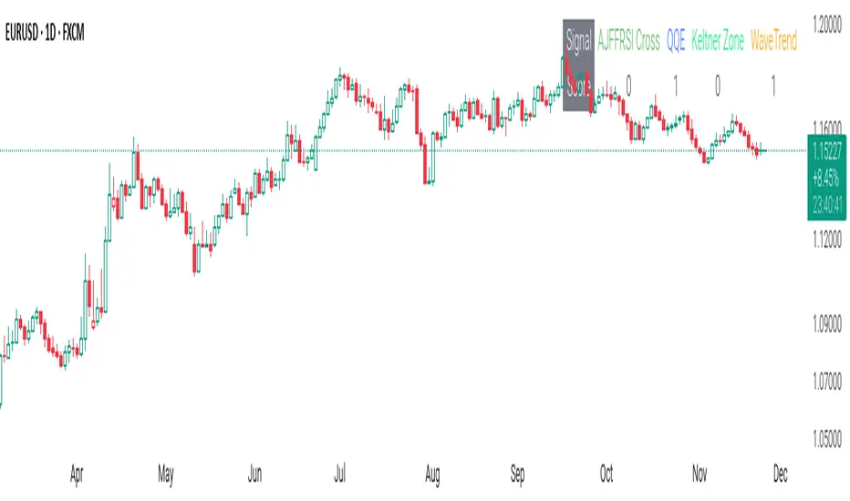
CSS_LFU_v0.1Overview:
A multi-factor, market-adaptive swing strategy designed for intraday and short-term crypto trading. It synthesizes momentum, volatility, and trend signals into a unified composite score over a configurable lookback window. The strategy leverages a modular, signal-weighted approach to ensure robust entry timing while remaining compatible with human-in-the-loop validation and algorithmic execution.
Core Modules:
AJFFRSI (RSX-based Momentum): Measures smoothed price momentum with noise-reduction filters to detect crossovers relative to the QQE trailing stop.
QQE (Quantitative Qualitative Easing RSI): A modified RSI with a dynamic trailing stop that adapts to short-term volatility, identifying exhaustion and potential reversal points.
Keltner Channel Zones: Determines overextension relative to trend, providing buy/sell zones based on ATR-banded EMA.
WaveTrend Oscillator: Confirms short-term swings and market direction through smoothed oscillator cross signals.
Rolling Composite Score: Aggregates module signals over a unified lookback (e.g., 144 bars) to normalize noise and capture consistent trends.
Signal Logic:
Each module outputs a discrete score (+1 / 0 / -1).
The rolling composite score sums all module scores over the lookback period.
Long positions trigger when the rolling score meets or exceeds the long threshold.
Short positions trigger when the rolling score meets or falls below the short threshold.
Multi-dimensional signal aggregation reduces false positives from single indicators.
Rolling lookback ensures score normalization across different volatility regimes.
Highly modular: easy to adapt modules or weights to different instruments or timeframes.
Fully compatible with automated execution pipelines, including custom exchange screener bots.
Use Case:
Ideal for quant-driven altcoin or multi-asset strategies where high-frequency validation is critical and sequential module weighting enhances trend flip detection.
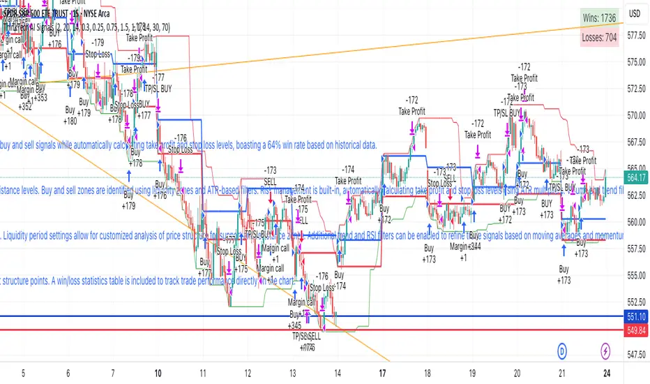
ThinkTech AI SignalsThink Tech AI Strategy
The Think Tech AI Strategy provides a structured approach to trading by integrating liquidity-based entries, ATR volatility thresholds, and dynamic risk management. This strategy generates buy and sell signals while automatically calculating take profit and stop loss levels, boasting a 64% win rate based on historical data.
Usage
The strategy can be used to identify key breakout and retest opportunities. Liquidity-based zones act as potential accumulation and distribution areas and may serve as future support or resistance levels. Buy and sell zones are identified using liquidity zones and ATR-based filters. Risk management is built-in, automatically calculating take profit and stop loss levels using ATR multipliers. Volume and trend filtering options help confirm directional bias using a 50 EMA and RSI filter. The strategy also allows for session-based trading, limiting trades to key market hours for higher probability setups.
Settings
The risk/reward ratio can be adjusted to define the desired stop loss and take profit calculations. The ATR length and threshold determine ATR-based breakout conditions for dynamic entries. Liquidity period settings allow for customized analysis of price structure for support and resistance zones. Additional trend and RSI filters can be enabled to refine trade signals based on moving averages and momentum conditions. A session filter is included to restrict trade signals to specific market hours.
Style
The strategy includes options to display liquidity lines, showing key support and resistance areas. The first 15-minute candle breakout zones can also be visualized to highlight critical market structure points. A win/loss statistics table is included to track trade performance directly on the chart.
This strategy is intended for descriptive analysis and should be used alongside other confluence factors. Optimize your trading process with Think Tech AI today!
Max Pain StrategyThe Max Pain Strategy uses a combination of volume and price movement thresholds to identify potential "pain zones" in the market. A "pain zone" is considered when the volume exceeds a certain multiple of its average over a defined lookback period, and the price movement exceeds a predefined percentage relative to the price at the beginning of the lookback period.
Here’s how the strategy functions step-by-step:
Inputs:
length: Defines the lookback period used to calculate the moving average of volume and the price change over that period.
volMultiplier: Sets a threshold multiplier for the volume; if the volume exceeds the average volume multiplied by this factor, it triggers the condition for a potential "pain zone."
priceMultiplier: Sets a threshold for the minimum percentage price change that is required for a "pain zone" condition.
Calculations:
averageVolume: The simple moving average (SMA) of volume over the specified lookback period.
priceChange: The absolute difference in price between the current bar's close and the close from the lookback period (length).
Pain Zone Condition:
The condition for entering a position is triggered if both the volume is higher than the average volume by the volMultiplier and the price change exceeds the price at the length-period ago by the priceMultiplier. This is an indication of significant market activity that could result in a price move.
Position Entry:
A long position is entered when the "pain zone" condition is met.
Exit Strategy:
The position is closed after the specified holdPeriods, which defines how many periods the position will be held after being entered.
Visualization:
A small triangle is plotted on the chart where the "pain zone" condition is met.
The background color changes to a semi-transparent red when the "pain zone" is active.
Scientific Explanation of the Components
Volume Analysis and Price Movement: These are two critical factors in trading strategies. Volume often serves as an indicator of market strength (or weakness), and price movement is a direct reflection of market sentiment. Higher volume with significant price movement may suggest that the market is entering a phase of increased volatility or trend formation, which the strategy aims to exploit.
Volume analysis: The study of volume as an indicator of market participation, with increased volume often signaling stronger trends (Murphy, J. J., Technical Analysis of the Financial Markets).
Price movement thresholds: A large price change over a short period may be interpreted as a breakout or a potential reversal point, aligning with volatility and liquidity analysis (Schwager, J. D., Market Wizards).
Repainting Check: This strategy does not involve any repainting because it is based on current and past data, and there is no reference to future values in the decision-making process. However, any strategy that uses lagging indicators or conditions based on historical bars, like close , is inherently a lagging strategy and might not predict real-time price action accurately until after the fact.
Risk Management: The position hold duration is predefined, which adds an element of time-based risk control. This duration ensures that the strategy does not hold a position indefinitely, which could expose it to unnecessary risk.
Potential Issues and Considerations
Repainting:
The strategy does not utilize future data or conditions that depend on future bars, so it does not inherently suffer from repainting issues.
However, since the strategy relies on volume and price change over a set lookback period, the decision to enter or exit a trade is only made after the data for the current bar is complete, meaning the trade decisions are somewhat delayed, which could be seen as a lagging feature rather than a repainting one.
Lagging Nature:
As with many technical analysis-based strategies, this one is based on past data (moving averages, price changes), meaning it reacts to market movements after they have already occurred, rather than predicting future price actions.
Overfitting Risk:
With parameters like the lookback period and multipliers being user-adjustable, there is a risk of overfitting to historical data. Adjusting parameters too much based on past performance can lead to poor out-of-sample results (Gauthier, P., Practical Quantitative Finance).
Conclusion
The Max Pain Strategy is a simple approach to identifying potential market entries based on volume spikes and significant price changes. It avoids repainting by relying solely on historical and current bar data, but it is inherently a lagging strategy that reacts to price and volume patterns after they have occurred. Therefore, the strategy can be effective in trending markets but may struggle in highly volatile, sideways markets.

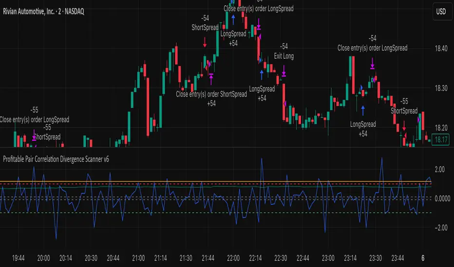
Profitable Pair Correlation Divergence Scanner v6This strategy identifies divergence opportunities between two correlated assets using a combination of Z-Score spread analysis, trend confirmation, RSI & MACD momentum checks, correlation filters, and ATR-based stop-loss/take-profit management. It’s optimized for positive P&L and realistic trade execution.
Key Features:
Pair Divergence Detection:
Measures deviation between returns of two assets and identifies overbought/oversold spread conditions using Z-Score.
Trend Alignment:
Trades only in the direction of the primary asset’s trend using a fast EMA vs slow EMA filter.
Momentum Confirmation:
Confirms trades with RSI and MACD to reduce false signals.
Correlation Filter:
Ensures the pair is strongly correlated before taking trades, avoiding noisy signals.
Risk Management:
Dynamic ATR-based stop-loss and take-profit ensures proper reward-to-risk ratio.
Exit Conditions:
Automatically closes positions when Z-Score normalizes, or ATR-based exits are hit.
How It Works:
Calculate Returns:
Computes returns for both assets over the selected timeframe.
Z-Score Spread:
Calculates the spread between returns and normalizes it using moving average and standard deviation.
Trend Filter:
Only takes long trades if the fast EMA is above the slow EMA, and short trades if the fast EMA is below the slow EMA.
Momentum Confirmation:
Confirms trade direction with RSI (>50 for longs, <50 for shorts) and MACD alignment.
Correlation Check:
Ensures the pair’s recent correlation is strong enough to validate divergence signals.
Trade Execution:
Opens positions when Z-Score crosses thresholds and all conditions align. Positions close when Z-Score normalizes or ATR-based SL/TP is hit.
Plot Explanation:
Z-Score: Blue line shows divergence magnitude.
Entry Levels: Red/Green lines mark long/short thresholds.
Exit Zone: Gray lines show normalization zone.
EMA Trend Lines: Purple (fast), Orange (slow) for trend alignment.
Correlation: Teal overlay shows current correlation strength.
Usage Tips:
Use highly correlated pairs for best results (e.g., EURUSD/GBPUSD).
Run on higher timeframe charts (1h or 4h) to reduce noise.
Adjust ATR multiplier based on volatility to avoid premature stops.
Combine with alerts for automated notifications or webhook execution.
Conclusion:
The Profitable Pair Correlation Divergence Scanner v6 is designed for traders who want systematic, low-risk, positive P&L trading opportunities with minimal manual monitoring. By combining trend alignment, momentum confirmation, correlation filters, and dynamic exits, it reduces false signals and improves execution reliability.
Run it on TradingView and watch how it captures divergence opportunities while maintaining positive P&L across trades.
Quasimodo Pattern Strategy Back Test [TradingFinder] QM Trading🔵 Introduction
The QM pattern, also known as the Quasimodo pattern, is one of the popular patterns in price action, and it is often used by technical analysts. The QM pattern is used to identify trend reversals and provides a very good risk-to-reward ratio. One of the advantages of the QM pattern is its high frequency and visibility in charts.
Additionally, due to its strength, it is highly profitable, and as mentioned, its risk-to-reward ratio is very good. The QM pattern is highly popular among traders in supply and demand, and traders also use this pattern.
The Price Action QM pattern, like other Price Action patterns, has two types: Bullish QM and Bearish QM patterns. To identify this pattern, you need to be familiar with its types to recognize it.
🔵 Identifying the QM Pattern
🟣 Bullish QM
In the bullish QM pattern, as you can see in the image below, an LL and HH are formed. As you can see, the neckline is marked as a dashed line. When the price reaches this range, it will start its upward movement.
🟣 Bearish QM
The Price Action QM pattern also has a bearish pattern. As you can see in the image below, initially, an HH and LL are formed. The neckline in this image is the dashed line, and when the LL is formed, the price reaches this neckline. However, it cannot pass it, and the downward trend resumes.
🔵 How to Use
The Quasimodo pattern is one of the clearest structures used to identify market reversals. It is built around the concept of a structural break followed by a pullback into an area of trapped liquidity. Instead of relying on lagging indicators, this pattern focuses purely on price action and how the market reacts after exhausting one side of liquidity. When understood correctly, it provides traders with precise entry points at the transition between trend phases.
🟣 Bullish Quasimodo
A bullish Quasimodo forms after a clear downtrend when sellers start losing control. The market continues to make lower lows until a sudden higher high appears, signaling that buyers are entering with strength. Price then pulls back to retest the previous low, creating what is known as the Quasimodo low.
This area often becomes the final trap for sellers before the market shifts upward. A visible rejection or displacement from this zone confirms bullish momentum. Traders usually place entries near this level, stops below the low, and targets at previous highs or the next resistance zone. Combining the setup with demand zones or Fair Value Gaps increases its accuracy.
🟣 Bearish Quasimodo
A bearish Quasimodo forms near the top of an uptrend when buyers begin to lose strength. The market continues to make higher highs until a sudden lower low breaks the bullish structure, showing that selling pressure is entering the market. Price then retraces upward to retest the previous high, forming the Quasimodo high, where breakout buyers are often trapped.
Once rejection appears at this level, it indicates a likely reversal. Traders can enter short near this area, with stop-losses placed above the high and targets near the next support or previous lows. The setup gains more reliability when aligned with supply zones, SMT divergence, or bearish Fair Value Gaps.
🔵 Setting
Pivot Period : You can use this parameter to use your desired period to identify the QM pattern. By default, this parameter is set to the number 5.
Take Profit Mode : You can choose your desired Take Profit in three ways. Based on the logic of the QM strategy, you can select two Take Profit levels, TP1 and TP2. You can also choose your take profit based on the Reward to Risk ratio. You must enter your desired R/R in the Reward to Risk Ratio parameter.
Stop Loss Refine : The loss limit of the QM strategy is based on its logic on the Head pattern. You can refine it using the ATR Refine option to prevent Stop Hunt. You can enter your desired coefficient in the Stop Loss ATR Adjustment Coefficient parameter.
Reward to Risk Ratio : If you set Take Profit Mode to R/R, you must enter your desired R/R here. For example, if your loss limit is 10 pips and you set R/R to 2, your take profit will be reached when the price is 20 pips away from your entry point.
Stop Loss ATR Adjustment Coefficient : If you set Stop Loss Refine to ATR Refine, you must adjust your loss limit coefficient here. For example, if your buy position's loss limit is at the price of 1000, and your ATR is 10, if you set Stop Loss ATR Adjustment Coefficient to 2, your loss limit will be at the price of 980.
Entry Level Validity : Determines how long the Entry level remains valid. The higher the level, the longer the entry level will remain valid. By default it is 2 and it can be set between 2 and 15.
🔵 Results
The following examples show the backtest results of the Quasimodo (QM) strategy in action. Each image is based on specific settings for the symbol, timeframe, and input parameters, illustrating how the QM logic can generate signals under different market conditions. The detailed configuration for each backtest is also displayed on the image.
⚠ Important Note : Even with identical settings and the same symbol, results may vary slightly across different brokers due to data feed variations and pricing differences.
Default Properties of Backtests :
OANDA:XAUUSD | TimeFrame: 5min | Duration: 1 Year :
BINANCE:BTCUSD | TimeFrame: 5min | Duration: 1 Year :
CAPITALCOM:US30 | TimeFrame: 5min | Duration: 1 Year :
NASDAQ:QQQ | TimeFrame: 5min | Duration: 5 Year :
OANDA:EURUSD | TimeFrame: 5min | Duration: 5 Year :
PEPPERSTONE:US500 | TimeFrame: 5min | Duration: 5 Year :

Enhanced OB Retest Strategy v7.0The OB Retest Strategy is a full Order Block retest trading system that detects, plots, and trades OB zones across multiple timeframes. It uses structure breaks, retrace depth, and ATR filters to identify strong reversal or continuation setups.
⸻
⚙️ Core Features
• Multi-timeframe OB detection using break-of-structure (BOS) logic
• Automatic zone creation for bullish and bearish order blocks
• Smart merging of overlapping OB zones
• Dynamic flip-zone logic that turns invalidated OBs into new zones
• Wick zone detection for high-precision entries
• ATR-based trailing stop and optional breakeven
• Adjustable retrace depth, breakout %, and ATR filters
• Built-in performance table showing PnL, win rate, and total trades
• Fully backtestable with date range and commission control
⸻
🧠 Logic Summary
1. Detects a BOS on the higher timeframe.
2. Identifies the last opposing candle as the valid OB.
3. Validates the OB based on ATR size and breakout strength.
4. Waits for price to retest the zone to a set depth.
5. Executes trades and manages exits using trailing stop or breakeven.
6. Flips invalidated zones automatically.
⸻
💡 Usage Tips
• Best used on 1H to 4H charts for swing setups.
• Tune ATR and breakout thresholds for your market’s volatility.
• Combine with higher-timeframe bias or liquidity levels for better accuracy.
⸻
⚠️ Notes
• For educational and testing purposes only.
• Backtested results do not predict future performance.
• Always test before live use.

Twisted Forex's Doji + Area StrategyTitle
Twisted Forex’s Doji + Area Strategy
Description
What this strategy does
This strategy looks for doji candles forming inside or near supply/demand areas . Areas are built from swing pivots and sized with ATR, then tracked for retests (“confirmations”). When a doji prints close to an area and quality checks pass, the strategy places a trade with the stop beyond the doji and a configurable R:R target.
How areas (zones) are built
• Swings are detected with a user-set pivot length.
• Each swing spawns a horizontal area centered at the pivot price with half-height = zoneHalfATR × ATR .
• Duplicates are de-duplicated by center distance (ATR-scaled).
• Areas fade when broken beyond a buffer or after an optional age (expiry).
• Retests are recorded when price touches and then bounces away from the area; repeated reactions increase the zone’s “strength”.
Signal logic (summary)
Doji detection: strict or loose body criteria with optional minimum wick fractions and ATR-scaled minimum range.
Proximity: price must be inside/near a supply or demand area (proxATR × ATR).
Side resolution: overlap is resolved by (a) which side price penetrates more, (b) fast/slow EMA trend, or (c) nearest distance. Optional “previous candle flip” can bias long after a bearish candle and short after a bullish one.
Optional 1-bar confirmation: the bar after the doji must close away from the area by confirmATR × ATR .
Quality filter (Off/Soft/Strict): four checks—(i) wick rejection past the edge, (ii) doji closes in an edge “band” of the area, (iii) fresh touch (cooldown), (iv) approach impulse over a short lookback. In Strict , thresholds auto-tighten.
Orders & exits
• Long: stop below doji low minus buffer; Short: above doji high plus buffer.
• Target = rrMultiple × risk distance .
• Pyramiding is off by default.
Position sizing
You can size from the script or from Strategy Properties:
• Script-driven (default): set Position sizing = “Risk % of equity” and choose riskPercent (e.g., 1.0%). The script applies safe floors/rounding (FX micro-lots by default) so quantity never rounds to zero.
• Properties-driven : toggle Use TV Properties → Order size ON, then pick “Percent of equity” in Properties (e.g., 1%). The header includes safe defaults so trades still place.
Key inputs to explore
• Zone building : pivotLen, zoneHalfATR, minDepartureATR, expiryBars, breakATR, leftBars, dedupeATR.
• Doji & proximity : strictDoji, dojiBodyFrac, minWickFrac, minRangeATR, proxATR, minBarsBetween.
• Overlap resolution : usePenetration, useTrend (EMA 21/55), “previous candle flip”, needNextBarConf & confirmATR.
• Quality : qualityMode (Off/Soft/Strict), minQualPass/kStrict, wickPenATR, edgeBandFrac, approachLookback, approachMinATR, freshTouchBars.
• Zone strength gating : minStrengthSoft / minStrengthStrict.
• HTF confluence (optional) : useHTFTrend (HTF EMA 34/89) and/or useHTFZoneProx (HTF swing bands).
Tips to make it cleaner / higher quality
• Turn needNextBarConf ON and use confirmATR = 0.10–0.15 .
• Increase approachMinATR (e.g., 0.35–0.45) to require a stronger pre-touch impulse.
• Raise minStrengthSoft/Strict (e.g., 4–6) so only well-reacted zones can signal.
• Use signalsOnlyConfirmed ON if you prefer trades only from zones with retests (the script falls back gracefully when none exist yet).
• Nudge proxATR to 0.5–0.6 to demand tighter proximity to the level.
• Optional: enable useHTFTrend to filter counter-trend setups.
Default settings used in this publication
• Initial capital: 100,000 (illustrative).
• Slippage: 1 tick; Commission: 0% (you can raise commission if you prefer—spread is partly modeled by slippage).
• Sizing: Risk % of equity via inputs; riskPercent = 1.0% ; FX uses micro-lot floors by default.
• Quality: Off by default (Soft/Strict available).
• HTF trend gate: Off by default.
Backtesting notes
For a meaningful sample size, test on liquid symbols/timeframes that yield 100+ trades (e.g., majors on 5–15m over 1–2 years). Backtests are modelled and broker costs/spread vary—validate on your feed and forward-test.
How to read the chart
Shaded bands are supply (above) and demand (below). Brighter bands are the nearest K per side (visual aid). BUY/SELL labels mark entries; colored dots show entry/SL/TP levels. You can hide zones or unconfirmed zones for a cleaner view.
Disclaimer
This is educational material, not financial advice. Trading involves risk. Always test and size responsibly.

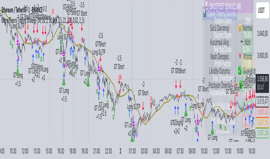
Game Theory Trading StrategyGame Theory Trading Strategy: Explanation and Working Logic
This Pine Script (version 5) code implements a trading strategy named "Game Theory Trading Strategy" in TradingView. Unlike the previous indicator, this is a full-fledged strategy with automated entry/exit rules, risk management, and backtesting capabilities. It uses Game Theory principles to analyze market behavior, focusing on herd behavior, institutional flows, liquidity traps, and Nash equilibrium to generate buy (long) and sell (short) signals. Below, I'll explain the strategy's purpose, working logic, key components, and usage tips in detail.
1. General Description
Purpose: The strategy identifies high-probability trading opportunities by combining Game Theory concepts (herd behavior, contrarian signals, Nash equilibrium) with technical analysis (RSI, volume, momentum). It aims to exploit market inefficiencies caused by retail herd behavior, institutional flows, and liquidity traps. The strategy is designed for automated trading with defined risk management (stop-loss/take-profit) and position sizing based on market conditions.
Key Features:
Herd Behavior Detection: Identifies retail panic buying/selling using RSI and volume spikes.
Liquidity Traps: Detects stop-loss hunting zones where price breaks recent highs/lows but reverses.
Institutional Flow Analysis: Tracks high-volume institutional activity via Accumulation/Distribution and volume spikes.
Nash Equilibrium: Uses statistical price bands to assess whether the market is in equilibrium or deviated (overbought/oversold).
Risk Management: Configurable stop-loss (SL) and take-profit (TP) percentages, dynamic position sizing based on Game Theory (minimax principle).
Visualization: Displays Nash bands, signals, background colors, and two tables (Game Theory status and backtest results).
Backtesting: Tracks performance metrics like win rate, profit factor, max drawdown, and Sharpe ratio.
Strategy Settings:
Initial capital: $10,000.
Pyramiding: Up to 3 positions.
Position size: 10% of equity (default_qty_value=10).
Configurable inputs for RSI, volume, liquidity, institutional flow, Nash equilibrium, and risk management.
Warning: This is a strategy, not just an indicator. It executes trades automatically in TradingView's Strategy Tester. Always backtest thoroughly and use proper risk management before live trading.
2. Working Logic (Step by Step)
The strategy processes each bar (candle) to generate signals, manage positions, and update performance metrics. Here's how it works:
a. Input Parameters
The inputs are grouped for clarity:
Herd Behavior (🐑):
RSI Period (14): For overbought/oversold detection.
Volume MA Period (20): To calculate average volume for spike detection.
Herd Threshold (2.0): Volume multiplier for detecting herd activity.
Liquidity Analysis (💧):
Liquidity Lookback (50): Bars to check for recent highs/lows.
Liquidity Sensitivity (1.5): Volume multiplier for trap detection.
Institutional Flow (🏦):
Institutional Volume Multiplier (2.5): For detecting large volume spikes.
Institutional MA Period (21): For Accumulation/Distribution smoothing.
Nash Equilibrium (⚖️):
Nash Period (100): For calculating price mean and standard deviation.
Nash Deviation (0.02): Multiplier for equilibrium bands.
Risk Management (🛡️):
Use Stop-Loss (true): Enables SL at 2% below/above entry price.
Use Take-Profit (true): Enables TP at 5% above/below entry price.
b. Herd Behavior Detection
RSI (14): Checks for extreme conditions:
Overbought: RSI > 70 (potential herd buying).
Oversold: RSI < 30 (potential herd selling).
Volume Spike: Volume > SMA(20) x 2.0 (herd_threshold).
Momentum: Price change over 10 bars (close - close ) compared to its SMA(20).
Herd Signals:
Herd Buying: RSI > 70 + volume spike + positive momentum = Retail buying frenzy (red background).
Herd Selling: RSI < 30 + volume spike + negative momentum = Retail selling panic (green background).
c. Liquidity Trap Detection
Recent Highs/Lows: Calculated over 50 bars (liquidity_lookback).
Psychological Levels: Nearest round numbers (e.g., $100, $110) as potential stop-loss zones.
Trap Conditions:
Up Trap: Price breaks recent high, closes below it, with a volume spike (volume > SMA x 1.5).
Down Trap: Price breaks recent low, closes above it, with a volume spike.
Visualization: Traps are marked with small red/green crosses above/below bars.
d. Institutional Flow Analysis
Volume Check: Volume > SMA(20) x 2.5 (inst_volume_mult) = Institutional activity.
Accumulation/Distribution (AD):
Formula: ((close - low) - (high - close)) / (high - low) * volume, cumulated over time.
Smoothed with SMA(21) (inst_ma_length).
Accumulation: AD > MA + high volume = Institutions buying.
Distribution: AD < MA + high volume = Institutions selling.
Smart Money Index: (close - open) / (high - low) * volume, smoothed with SMA(20). Positive = Smart money buying.
e. Nash Equilibrium
Calculation:
Price mean: SMA(100) (nash_period).
Standard deviation: stdev(100).
Upper Nash: Mean + StdDev x 0.02 (nash_deviation).
Lower Nash: Mean - StdDev x 0.02.
Conditions:
Near Equilibrium: Price between upper and lower Nash bands (stable market).
Above Nash: Price > upper band (overbought, sell potential).
Below Nash: Price < lower band (oversold, buy potential).
Visualization: Orange line (mean), red/green lines (upper/lower bands).
f. Game Theory Signals
The strategy generates three types of signals, combined into long/short triggers:
Contrarian Signals:
Buy: Herd selling + (accumulation or down trap) = Go against retail panic.
Sell: Herd buying + (distribution or up trap).
Momentum Signals:
Buy: Below Nash + positive smart money + no herd buying.
Sell: Above Nash + negative smart money + no herd selling.
Nash Reversion Signals:
Buy: Below Nash + rising close (close > close ) + volume > MA.
Sell: Above Nash + falling close + volume > MA.
Final Signals:
Long Signal: Contrarian buy OR momentum buy OR Nash reversion buy.
Short Signal: Contrarian sell OR momentum sell OR Nash reversion sell.
g. Position Management
Position Sizing (Minimax Principle):
Default: 1.0 (10% of equity).
In Nash equilibrium: Reduced to 0.5 (conservative).
During institutional volume: Increased to 1.5 (aggressive).
Entries:
Long: If long_signal is true and no existing long position (strategy.position_size <= 0).
Short: If short_signal is true and no existing short position (strategy.position_size >= 0).
Exits:
Stop-Loss: If use_sl=true, set at 2% below/above entry price.
Take-Profit: If use_tp=true, set at 5% above/below entry price.
Pyramiding: Up to 3 concurrent positions allowed.
h. Visualization
Nash Bands: Orange (mean), red (upper), green (lower).
Background Colors:
Herd buying: Red (90% transparency).
Herd selling: Green.
Institutional volume: Blue.
Signals:
Contrarian buy/sell: Green/red triangles below/above bars.
Liquidity traps: Red/green crosses above/below bars.
Tables:
Game Theory Table (Top-Right):
Herd Behavior: Buying frenzy, selling panic, or normal.
Institutional Flow: Accumulation, distribution, or neutral.
Nash Equilibrium: In equilibrium, above, or below.
Liquidity Status: Trap detected or safe.
Position Suggestion: Long (green), Short (red), or Wait (gray).
Backtest Table (Bottom-Right):
Total Trades: Number of closed trades.
Win Rate: Percentage of winning trades.
Net Profit/Loss: In USD, colored green/red.
Profit Factor: Gross profit / gross loss.
Max Drawdown: Peak-to-trough equity drop (%).
Win/Loss Trades: Number of winning/losing trades.
Risk/Reward Ratio: Simplified Sharpe ratio (returns / drawdown).
Avg Win/Loss Ratio: Average win per trade / average loss per trade.
Last Update: Current time.
i. Backtesting Metrics
Tracks:
Total trades, winning/losing trades.
Win rate (%).
Net profit ($).
Profit factor (gross profit / gross loss).
Max drawdown (%).
Simplified Sharpe ratio (returns / drawdown).
Average win/loss ratio.
Updates metrics on each closed trade.
Displays a label on the last bar with backtest period, total trades, win rate, and net profit.
j. Alerts
No explicit alertconditions defined, but you can add them for long_signal and short_signal (e.g., alertcondition(long_signal, "GT Long Entry", "Long Signal Detected!")).
Use TradingView's alert system with Strategy Tester outputs.
3. Usage Tips
Timeframe: Best for H1-D1 timeframes. Shorter frames (M1-M15) may produce noisy signals.
Settings:
Risk Management: Adjust sl_percent (e.g., 1% for volatile markets) and tp_percent (e.g., 3% for scalping).
Herd Threshold: Increase to 2.5 for stricter herd detection in choppy markets.
Liquidity Lookback: Reduce to 20 for faster markets (e.g., crypto).
Nash Period: Increase to 200 for longer-term analysis.
Backtesting:
Use TradingView's Strategy Tester to evaluate performance.
Check win rate (>50%), profit factor (>1.5), and max drawdown (<20%) for viability.
Test on different assets/timeframes to ensure robustness.
Live Trading:
Start with a demo account.
Combine with other indicators (e.g., EMAs, support/resistance) for confirmation.
Monitor liquidity traps and institutional flow for context.
Risk Management:
Always use SL/TP to limit losses.
Adjust position_size for risk tolerance (e.g., 5% of equity for conservative trading).
Avoid over-leveraging (pyramiding=3 can amplify risk).
Troubleshooting:
If no trades are executed, check signal conditions (e.g., lower herd_threshold or liquidity_sensitivity).
Ensure sufficient historical data for Nash and liquidity calculations.
If tables overlap, adjust position.top_right/bottom_right coordinates.
4. Key Differences from the Previous Indicator
Indicator vs. Strategy: The previous code was an indicator (VP + Game Theory Integrated Strategy) focused on visualization and alerts. This is a strategy with automated entries/exits and backtesting.
Volume Profile: Absent in this strategy, making it lighter but less focused on high-volume zones.
Wick Analysis: Not included here, unlike the previous indicator's heavy reliance on wick patterns.
Backtesting: This strategy includes detailed performance metrics and a backtest table, absent in the indicator.
Simpler Signals: Focuses on Game Theory signals (contrarian, momentum, Nash reversion) without the "Power/Ultra Power" hierarchy.
Risk Management: Explicit SL/TP and dynamic position sizing, not present in the indicator.
5. Conclusion
The "Game Theory Trading Strategy" is a sophisticated system leveraging herd behavior, institutional flows, liquidity traps, and Nash equilibrium to trade market inefficiencies. It’s designed for traders who understand Game Theory principles and want automated execution with robust risk management. However, it requires thorough backtesting and parameter optimization for specific markets (e.g., forex, crypto, stocks). The backtest table and visual aids make it easy to monitor performance, but always combine with other analysis tools and proper capital management.
If you need help with backtesting, adding alerts, or optimizing parameters, let me know!
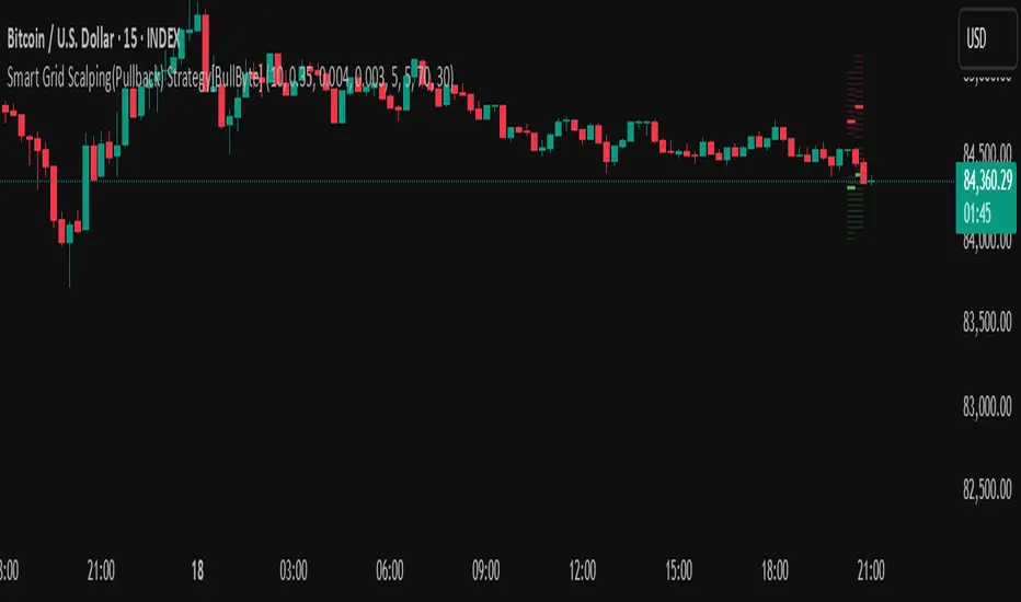
Smart Grid Scalping (Pullback) Strategy[BullByte]The Smart Grid Scalping (Pullback) Strategy is a high-frequency trading strategy designed for short-term traders who seek to capitalize on market pullbacks. This strategy utilizes a dynamic ATR-based grid system to define optimal entry points, ensuring precise trade execution. It integrates volatility filtering and an RSI-based confirmation mechanism to enhance signal accuracy and reduce false entries.
This strategy is specifically optimized for scalping by dynamically adjusting trade levels based on current market conditions. The grid-based system helps capture retracement opportunities while maintaining strict trade management through predefined profit targets and trailing stop-loss mechanisms.
Key Features :
1. ATR-Based Grid System :
- Uses a 10-period ATR to dynamically calculate grid levels for entry points.
- Prevents chasing trades by ensuring price has reached key levels before executing entries.
2. No Trade Zone Protection :
- Avoids low-volatility zones where price action is indecisive.
- Ensures only high-momentum trades are executed to improve success rate.
3. RSI-Based Entry Confirmation :
- Long trades are triggered when RSI is below 30 (oversold) and price is in the lower grid zone.
- Short trades are triggered when RSI is above 70 (overbought) and price is in the upper grid zone.
4. Automated Trade Execution :
- Long Entry: Triggered when price drops below the first grid level with sufficient volatility.
- Short Entry: Triggered when price exceeds the highest grid level with sufficient volatility.
5. Take Profit & Trailing Stop :
- Profit target set at a customizable percentage (default 0.2%).
- Adaptive trailing stop mechanism using ATR to lock in profits while minimizing premature exits.
6. Visual Trade Annotations :
- Clearly labeled "LONG" and "SHORT" markers appear at trade entries for better visualization.
- Grid levels are plotted dynamically to aid decision-making.
Strategy Logic :
- The script first calculates the ATR-based grid levels and ensures price action has sufficient volatility before allowing trades.
- An additional RSI filter is used to ensure trades are taken at ideal market conditions.
- Once a trade is executed, the script implements a trailing stop and predefined take profit to maximize gains while reducing risks.
---
Disclaimer :
Risk Warning :
This strategy is provided for educational and informational purposes only. Trading involves significant risk, and past performance is not indicative of future results. Users are advised to conduct their own due diligence and risk management before using this strategy in live trading.
The developer and publisher of this script are not responsible for any financial losses incurred by the use of this strategy. Market conditions, slippage, and execution quality can affect real-world trading outcomes.
Use this script at your own discretion and always trade responsibly.
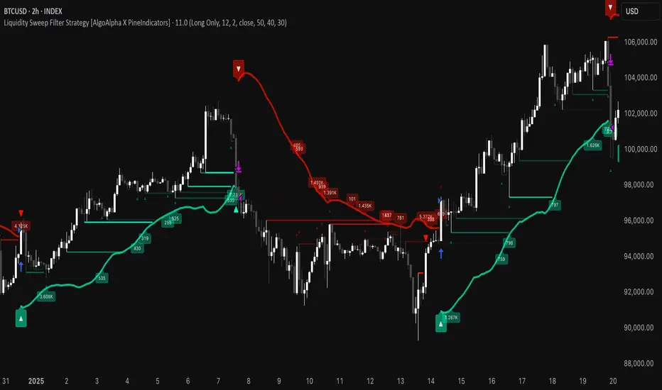
Liquidity Sweep Filter Strategy [AlgoAlpha X PineIndicators]This strategy is based on the Liquidity Sweep Filter developed by AlgoAlpha. Full credit for the concept and original indicator goes to AlgoAlpha.
The Liquidity Sweep Filter Strategy is a non-repainting trading system designed to identify liquidity sweeps, trend shifts, and high-impact price levels. It incorporates volume-based liquidation analysis, trend confirmation, and dynamic support/resistance detection to optimize trade entries and exits.
This strategy helps traders:
Detect liquidity sweeps where major market participants trigger stop losses and liquidations.
Identify trend shifts using a volatility-based moving average system.
Analyze volume distribution with a built-in volume profile visualization.
Filter noise by differentiating between major and minor liquidity sweeps.
How the Liquidity Sweep Filter Strategy Works
1. Trend Detection Using Volatility-Based Filtering
The strategy applies a volatility-adjusted moving average system to determine trend direction:
A central trend line is calculated using an EMA smoothed over a user-defined length.
Upper and lower deviation bands are created based on the average price deviation over multiple periods.
If price closes above the upper band, the strategy signals an uptrend.
If price closes below the lower band, the strategy signals a downtrend.
This approach ensures that trend shifts are confirmed only when price significantly moves beyond normal market fluctuations.
2. Liquidity Sweep Detection
Liquidity sweeps occur when price temporarily breaks key levels, triggering stop-loss liquidations or margin call events. The strategy tracks swing highs and lows, marking potential liquidity grabs:
Bearish Liquidity Sweeps – Price breaks a recent high, then reverses downward.
Bullish Liquidity Sweeps – Price breaks a recent low, then reverses upward.
Volume Integration – The strategy analyzes trading volume at each sweep to differentiate between major and minor sweeps.
Key levels where liquidity sweeps occur are plotted as color-coded horizontal lines:
Red lines indicate bearish liquidity sweeps.
Green lines indicate bullish liquidity sweeps.
Labels are displayed at each sweep, showing the volume of liquidated positions at that level.
3. Volume Profile Analysis
The strategy includes an optional volume profile visualization, displaying how trading volume is distributed across different price levels.
Features of the volume profile:
Point of Control (POC) – The price level with the highest traded volume is marked as a key area of interest.
Bounding Box – The profile is enclosed within a transparent box, helping traders visualize the price range of high trading activity.
Customizable Resolution & Scale – Traders can adjust the granularity of the profile to match their preferred time frame.
The volume profile helps identify zones of strong support and resistance, making it easier to anticipate price reactions at key levels.
Trade Entry & Exit Conditions
The strategy allows traders to configure trade direction:
Long Only – Only takes long trades.
Short Only – Only takes short trades.
Long & Short – Trades in both directions.
Entry Conditions
Long Entry:
A bullish trend shift is confirmed.
A bullish liquidity sweep occurs (price sweeps below a key level and reverses).
The trade direction setting allows long trades.
Short Entry:
A bearish trend shift is confirmed.
A bearish liquidity sweep occurs (price sweeps above a key level and reverses).
The trade direction setting allows short trades.
Exit Conditions
Closing a Long Position:
A bearish trend shift occurs.
The position is liquidated at a predefined liquidity sweep level.
Closing a Short Position:
A bullish trend shift occurs.
The position is liquidated at a predefined liquidity sweep level.
Customization Options
The strategy offers multiple adjustable settings:
Trade Mode: Choose between Long Only, Short Only, or Long & Short.
Trend Calculation Length & Multiplier: Adjust how trend signals are calculated.
Liquidity Sweep Sensitivity: Customize how aggressively the strategy identifies sweeps.
Volume Profile Display: Enable or disable the volume profile visualization.
Bounding Box & Scaling: Control the size and position of the volume profile.
Color Customization: Adjust colors for bullish and bearish signals.
Considerations & Limitations
Liquidity sweeps do not always result in reversals. Some price sweeps may continue in the same direction.
Works best in volatile markets. In low-volatility environments, liquidity sweeps may be less reliable.
Trend confirmation adds a slight delay. The strategy ensures valid signals, but this may result in slightly later entries.
Large volume imbalances may distort the volume profile. Adjusting the scale settings can help improve visualization.
Conclusion
The Liquidity Sweep Filter Strategy is a volume-integrated trading system that combines liquidity sweeps, trend analysis, and volume profile data to optimize trade execution.
By identifying key price levels where liquidations occur, this strategy provides valuable insight into market behavior, helping traders make better-informed trading decisions.
Key use cases for this strategy:
Liquidity-Based Trading – Capturing moves triggered by stop hunts and liquidations.
Volume Analysis – Using volume profile data to confirm high-activity price zones.
Trend Following – Entering trades based on confirmed trend shifts.
Support & Resistance Trading – Using liquidity sweep levels as dynamic price zones.
This strategy is fully customizable, allowing traders to adapt it to different market conditions, timeframes, and risk preferences.
Full credit for the original concept and indicator goes to AlgoAlpha.
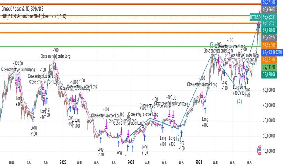
NUTJP CDC ActionZone 20241. Core Components of the Strategy
• Fast EMA and Slow EMA:
• The Fast EMA (shorter period) is more reactive to recent price changes.
• The Slow EMA (longer period) reacts slower and provides a smoother view of the overall trend.
• Relationship Between Fast EMA and Slow EMA:
• When the Fast EMA is above the Slow EMA, the market is considered Bullish.
• When the Fast EMA is below the Slow EMA, the market is considered Bearish.
2. Zones Based on Price and EMAs
The strategy defines six zones based on the position of the price, Fast EMA, and Slow EMA:
1. Green Zone (Buy):
• Bullish trend (Fast EMA > Slow EMA)
• Price is above the Fast EMA.
• Indicates a strong uptrend and suggests buying.
2. Blue and Light Blue Zones (Pre-Buy):
• Price is above the Fast EMA but below or near the Slow EMA.
• Represents potential bullish signals but not strong enough to trigger a buy.
3. Red Zone (Sell):
• Bearish trend (Fast EMA < Slow EMA)
• Price is below the Fast EMA.
• Indicates a strong downtrend and suggests selling or avoiding long trades.
4. Orange and Yellow Zones (Pre-Sell):
• Price is below the Fast EMA but above or near the Slow EMA.
• Represents potential bearish signals but not strong enough to trigger a sell.
These zones help traders visualize the market conditions and determine whether to buy, hold, or sell.
3. Buy and Sell Conditions
• Buy Condition:
A buy signal is triggered when:
• The price enters the Green Zone (Bullish trend and price > Fast EMA).
• It’s the first green candle after a non-green candle.
• Sell Condition:
A sell signal is triggered when:
• The price enters the Red Zone (Bearish trend and price < Fast EMA).
• It’s the first red candle after a non-red candle.
4. Trade Execution Logic
• Buy:
The strategy enters a long position (buy) when the above buy condition is met.
• Sell:
The strategy exits the long position when the sell condition is met.
Note: It doesn’t support short trades, meaning it doesn’t enter sell positions.
5. Momentum-Based Signals (Optional)
The indicator also includes momentum signals using Stochastic RSI to provide additional buy/sell signals:
• These are based on oversold and overbought levels of the Stochastic RSI.
• It filters signals depending on whether the trend is Bullish or Bearish.
6. Visual Features
The indicator is designed to make the trading zones and signals visually intuitive:
• Bar Colors:
Candlesticks are colored based on the current zone (e.g., Green for Buy, Red for Sell).
• EMA Lines:
The Fast EMA and Slow EMA are plotted, making it easy to see crossover points.
• Buy/Sell Signals:
Marked with shapes (e.g., circles) below/above bars for clarity.
7. Strategy Assumptions
• Trend-Following Nature:
This strategy assumes that trends persist. It works best in trending markets but might give false signals in ranging markets.
• Lagging Nature of EMAs:
As EMAs are lagging indicators, buy and sell signals may occur after significant moves have already begun or ended.
• Momentum Confirmation (Optional):
Adding momentum signals can help filter false signals, though it’s not part of the core logic.
8. Usage Recommendations
• Timeframes:
Works on various timeframes but may perform better on higher timeframes (e.g., 1H, Daily) to reduce noise.
• Markets:
Can be applied to stocks, forex, and cryptocurrencies.
• Backtesting and Optimization:
Before live trading, backtest the strategy with different EMA periods and other parameters to find optimal settings for your market and timeframe.
Mirror Blocks: StrategyMirror Blocks is an educational structural-wave model built around a unique concept:
the interaction of mirrored weighted moving averages (“blocks”) that reflect shifts in market structure as price transitions between layered symmetry zones.
Rather than attempting to “predict” markets, the Mirror Blocks framework visualizes how price behaves when it expands away from, contracts toward, or flips across stacked WMA structures. These mirrored layers form a wave-like block system that highlights transitional zones in a clean, mechanical way.
This strategy version allows you to study how these structural transitions behave in different environments and on different timeframes.
The goal is understanding wave structure, not generating signals.
How It Works
Mirror Blocks builds three mirrored layers:
Top Block (Structural High Symmetry)
Base Block (Neutral Wave)
Bottom Block (Structural Low Symmetry)
The relative position of these blocks — and how price interacts with them — helps visualize:
Compression and expansion
Reversal zones
Wave stability
Momentum transitions
Structure flips
A structure is considered bullish-stack aligned when:
Top > Base > Bottom
and bearish-stack aligned when:
Bottom > Base > Top
These formations create the core of the Mirror Blocks wave engine.
What the Strategy Version Adds
This version includes:
Long Only, Short Only, or Long & Short modes
Adjustable symmetry distance (Mirror Distance)
Configurable WMA smoothing length
Optional trend filter using fast/slow MA comparison
ENTER / EXIT / LONG / SHORT labels for structural transitions
Fixed stop-loss controls for research
A clean, transparent structure with no hidden components
It is optimized for educational chart study, not automated signals.
Intended Purpose
Mirror Blocks is meant to help traders:
Study structural transitions
Understand symmetry-based wave models
Explore how price interacts with mirrored layers
Examine reversals and expansions from a mechanical perspective
Conduct long and short backtesting for research
Develop a deeper sense of market rhythm
This is not a prediction model.
It is a visual and structural framework for understanding movement.
Backtesting Disclaimer
Backtest results can vary depending on:
Slippage settings
Commission settings
Timeframe
Asset volatility
Structural sensitivity parameters
Past performance does not guarantee future results.
Use this as a research tool only.
Warnings & Compliance
This script is educational.
It is not financial advice.
It does not provide signals.
It does not promise profitability.
The purpose is to help visualize structure, not predict price.
The strategy features are simply here to help users study how structural transitions behave under various conditions.
License
Released under the Michael Culpepper Gratitude License (2025).
Use and modify freely for education and research with attribution.
No resale.
No promises of profitability.
Purpose is understanding, not signals.
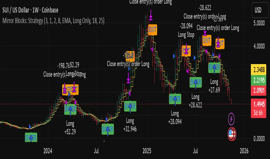
W%R Pullback+EMA Trend [TS_Indie]🔰 Core Concept of the Strategy
The main idea is “Trend-Following with Momentum Pullback.”
This means trading in the direction of the main trend (defined by EMA) while using Williams %R to identify pullback entries (buying the dip or selling the rally) where momentum returns to the trend direction.
📊 Indicators Used
1. EMA Fast – Defines the short-term trend.
2. EMA Slow – Defines the long-term trend (used as a trend filter).
3. Williams %R
• Overbought zone: above -20
• Oversold zone: below -80
⚙️ Entry Rules
🔹 Buy Setup
1. EMA Fast > EMA Slow → Uptrend condition.
2. Williams %R on the previous candle dropped below -80, and on the current candle, it crosses back above -80 → indicates momentum returning to the upside.
3. Current close is above EMA Fast.
4. Entry Buy at the close of the candle where %R crosses above -80.
🎯 Entry, Stop Loss, and Take Profit
1. Entry : At the candle close where the signal occurs.
2. Stop Loss : At the lowest low between the current and previous candles.
3. Take Profit : Calculated based on entry price and stop loss distance multiplied by the Risk/Reward Ratio.
🔹 Sell Setup
1. EMA Fast < EMA Slow → Downtrend condition.
2. Williams %R on the previous candle went above -20, and on the current candle, it crosses back below -20 → indicates renewed selling momentum.
3. Current price is below EMA Fast.
4. Entry Sell at the close of the candle where %R crosses below -20.
🎯 Entry, Stop Loss, and Take Profit
1. Entry : At the candle close where the signal occurs.
2. Stop Loss : At the highest high between the current and previous candles.
3. Take Profit : Calculated based on entry price and stop loss distance multiplied by the Risk/Reward Ratio.
⚙️ Optional Parameters
• Custom Risk/Reward Ratio for Take Profit.
• Option to add ATR buffer to Stop Loss.
• Adjustable EMA Fast period.
• Adjustable EMA Slow period.
• Adjustable Williams %R period.
• Option to enable Long only / Short only positions.
• Customizable Backtest start and end date.
• Customizable trading session time.
⏰ Alert Function
Alerts display:
• Entry price
• Stop Loss price
• Take Profit price
Guys, try adjusting the parameters yourselves!
I’ve been tweaking the settings for several days and managed to get great results on XAU/USD in the 5-minute timeframe.
I think this strategy is quite interesting and could potentially deliver good results on other instruments as well.
⚠️ Disclaimer
This indicator is designed for educational and research purposes only.
It does not guarantee profits and should not be considered financial advice.
Trading in financial markets involves significant risk, including the potential loss of capital.
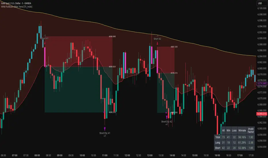
Anomalous Holonomy Field Theory🌌 Anomalous Holonomy Field Theory (AHFT) - Revolutionary Quantum Market Analysis
Where Theoretical Physics Meets Trading Reality
A Groundbreaking Synthesis of Differential Geometry, Quantum Field Theory, and Market Dynamics
🔬 THEORETICAL FOUNDATION - THE MATHEMATICS OF MARKET REALITY
The Anomalous Holonomy Field Theory represents an unprecedented fusion of advanced mathematical physics with practical market analysis. This isn't merely another indicator repackaging old concepts - it's a fundamentally new lens through which to view and understand market structure .
1. HOLONOMY GROUPS (Differential Geometry)
In differential geometry, holonomy measures how vectors change when parallel transported around closed loops in curved space. Applied to markets:
Mathematical Formula:
H = P exp(∮_C A_μ dx^μ)
Where:
P = Path ordering operator
A_μ = Market connection (price-volume gauge field)
C = Closed price path
Market Implementation:
The holonomy calculation measures how price "remembers" its journey through market space. When price returns to a previous level, the holonomy captures what has changed in the market's internal geometry. This reveals:
Hidden curvature in the market manifold
Topological obstructions to arbitrage
Geometric phase accumulated during price cycles
2. ANOMALY DETECTION (Quantum Field Theory)
Drawing from the Adler-Bell-Jackiw anomaly in quantum field theory:
Mathematical Formula:
∂_μ j^μ = (e²/16π²)F_μν F̃^μν
Where:
j^μ = Market current (order flow)
F_μν = Field strength tensor (volatility structure)
F̃^μν = Dual field strength
Market Application:
Anomalies represent symmetry breaking in market structure - moments when normal patterns fail and extraordinary opportunities arise. The system detects:
Spontaneous symmetry breaking (trend reversals)
Vacuum fluctuations (volatility clusters)
Non-perturbative effects (market crashes/melt-ups)
3. GAUGE THEORY (Theoretical Physics)
Markets exhibit gauge invariance - the fundamental physics remains unchanged under certain transformations:
Mathematical Formula:
A'_μ = A_μ + ∂_μΛ
This ensures our signals are gauge-invariant observables , immune to arbitrary market "coordinate changes" like gaps or reference point shifts.
4. TOPOLOGICAL DATA ANALYSIS
Using persistent homology and Morse theory:
Mathematical Formula:
β_k = dim(H_k(X))
Where β_k are the Betti numbers describing topological features that persist across scales.
🎯 REVOLUTIONARY SIGNAL CONFIGURATION
Signal Sensitivity (0.5-12.0, default 2.5)
Controls the responsiveness of holonomy field calculations to market conditions. This parameter directly affects the threshold for detecting quantum phase transitions in price action.
Optimization by Timeframe:
Scalping (1-5min): 1.5-3.0 for rapid signal generation
Day Trading (15min-1H): 2.5-5.0 for balanced sensitivity
Swing Trading (4H-1D): 5.0-8.0 for high-quality signals only
Score Amplifier (10-200, default 50)
Scales the raw holonomy field strength to produce meaningful signal values. Higher values amplify weak signals in low-volatility environments.
Signal Confirmation Toggle
When enabled, enforces additional technical filters (EMA and RSI alignment) to reduce false positives. Essential for conservative strategies.
Minimum Bars Between Signals (1-20, default 5)
Prevents overtrading by enforcing quantum decoherence time between signals. Higher values reduce whipsaws in choppy markets.
👑 ELITE EXECUTION SYSTEM
Execution Modes:
Conservative Mode:
Stricter signal criteria
Higher quality thresholds
Ideal for stable market conditions
Adaptive Mode:
Self-adjusting parameters
Balances signal frequency with quality
Recommended for most traders
Aggressive Mode:
Maximum signal sensitivity
Captures rapid market moves
Best for experienced traders in volatile conditions
Dynamic Position Sizing:
When enabled, the system scales position size based on:
Holonomy field strength
Current volatility regime
Recent performance metrics
Advanced Exit Management:
Implements trailing stops based on ATR and signal strength, with mode-specific multipliers for optimal profit capture.
🧠 ADAPTIVE INTELLIGENCE ENGINE
Self-Learning System:
The strategy analyzes recent trade outcomes and adjusts:
Risk multipliers based on win/loss ratios
Signal weights according to performance
Market regime detection for environmental adaptation
Learning Speed (0.05-0.3):
Controls adaptation rate. Higher values = faster learning but potentially unstable. Lower values = stable but slower adaptation.
Performance Window (20-100 trades):
Number of recent trades analyzed for adaptation. Longer windows provide stability, shorter windows increase responsiveness.
🎨 REVOLUTIONARY VISUAL SYSTEM
1. Holonomy Field Visualization
What it shows: Multi-layer quantum field bands representing market resonance zones
How to interpret:
Blue/Purple bands = Primary holonomy field (strongest resonance)
Band width = Field strength and volatility
Price within bands = Normal quantum state
Price breaking bands = Quantum phase transition
Trading application: Trade reversals at band extremes, breakouts on band violations with strong signals.
2. Quantum Portals
What they show: Entry signals with recursive depth patterns indicating momentum strength
How to interpret:
Upward triangles with portals = Long entry signals
Downward triangles with portals = Short entry signals
Portal depth = Signal strength and expected momentum
Color intensity = Probability of success
Trading application: Enter on portal appearance, with size proportional to portal depth.
3. Field Resonance Bands
What they show: Fibonacci-based harmonic price zones where quantum resonance occurs
How to interpret:
Dotted circles = Minor resonance levels
Solid circles = Major resonance levels
Color coding = Resonance strength
Trading application: Use as dynamic support/resistance, expect reactions at resonance zones.
4. Anomaly Detection Grid
What it shows: Fractal-based support/resistance with anomaly strength calculations
How to interpret:
Triple-layer lines = Major fractal levels with high anomaly probability
Labels show: Period (H8-H55), Price, and Anomaly strength (φ)
⚡ symbol = Extreme anomaly detected
● symbol = Strong anomaly
○ symbol = Normal conditions
Trading application: Expect major moves when price approaches high anomaly levels. Use for precise entry/exit timing.
5. Phase Space Flow
What it shows: Background heatmap revealing market topology and energy
How to interpret:
Dark background = Low market energy, range-bound
Purple glow = Building energy, trend developing
Bright intensity = High energy, strong directional move
Trading application: Trade aggressively in bright phases, reduce activity in dark phases.
📊 PROFESSIONAL DASHBOARD METRICS
Holonomy Field Strength (-100 to +100)
What it measures: The Wilson loop integral around price paths
>70: Strong positive curvature (bullish vortex)
<-70: Strong negative curvature (bearish collapse)
Near 0: Flat connection (range-bound)
Anomaly Level (0-100%)
What it measures: Quantum vacuum expectation deviation
>70%: Major anomaly (phase transition imminent)
30-70%: Moderate anomaly (elevated volatility)
<30%: Normal quantum fluctuations
Quantum State (-1, 0, +1)
What it measures: Market wave function collapse
+1: Bullish eigenstate |↑⟩
0: Superposition (uncertain)
-1: Bearish eigenstate |↓⟩
Signal Quality Ratings
LEGENDARY: All quantum fields aligned, maximum probability
EXCEPTIONAL: Strong holonomy with anomaly confirmation
STRONG: Good field strength, moderate anomaly
MODERATE: Decent signals, some uncertainty
WEAK: Minimal edge, high quantum noise
Performance Metrics
Win Rate: Rolling performance with emoji indicators
Daily P&L: Real-time profit tracking
Adaptive Risk: Current risk multiplier status
Market Regime: Bull/Bear classification
🏆 WHY THIS CHANGES EVERYTHING
Traditional technical analysis operates on 100-year-old principles - moving averages, support/resistance, and pattern recognition. These work because many traders use them, creating self-fulfilling prophecies.
AHFT transcends this limitation by analyzing markets through the lens of fundamental physics:
Markets have geometry - The holonomy calculations reveal this hidden structure
Price has memory - The geometric phase captures path-dependent effects
Anomalies are predictable - Quantum field theory identifies symmetry breaking
Everything is connected - Gauge theory unifies disparate market phenomena
This isn't just a new indicator - it's a new way of thinking about markets . Just as Einstein's relativity revolutionized physics beyond Newton's mechanics, AHFT revolutionizes technical analysis beyond traditional methods.
🔧 OPTIMAL SETTINGS FOR MNQ 10-MINUTE
For the Micro E-mini Nasdaq-100 on 10-minute timeframe:
Signal Sensitivity: 2.5-3.5
Score Amplifier: 50-70
Execution Mode: Adaptive
Min Bars Between: 3-5
Theme: Quantum Nebula or Dark Matter
💭 THE JOURNEY - FROM IMPOSSIBLE THEORY TO TRADING REALITY
Creating AHFT was a mathematical odyssey that pushed the boundaries of what's possible in Pine Script. The journey began with a seemingly impossible question: Could the profound mathematical structures of theoretical physics be translated into practical trading tools?
The Theoretical Challenge:
Months were spent diving deep into differential geometry textbooks, studying the works of Chern, Simons, and Witten. The mathematics of holonomy groups and gauge theory had never been applied to financial markets. Translating abstract mathematical concepts like parallel transport and fiber bundles into discrete price calculations required novel approaches and countless failed attempts.
The Computational Nightmare:
Pine Script wasn't designed for quantum field theory calculations. Implementing the Wilson loop integral, managing complex array structures for anomaly detection, and maintaining computational efficiency while calculating geometric phases pushed the language to its limits. There were moments when the entire project seemed impossible - the script would timeout, produce nonsensical results, or simply refuse to compile.
The Breakthrough Moments:
After countless sleepless nights and thousands of lines of code, breakthrough came through elegant simplifications. The realization that market anomalies follow patterns similar to quantum vacuum fluctuations led to the revolutionary anomaly detection system. The discovery that price paths exhibit holonomic memory unlocked the geometric phase calculations.
The Visual Revolution:
Creating visualizations that could represent 4-dimensional quantum fields on a 2D chart required innovative approaches. The multi-layer holonomy field, recursive quantum portals, and phase space flow representations went through dozens of iterations before achieving the perfect balance of beauty and functionality.
The Balancing Act:
Perhaps the greatest challenge was maintaining mathematical rigor while ensuring practical trading utility. Every formula had to be both theoretically sound and computationally efficient. Every visual had to be both aesthetically pleasing and information-rich.
The result is more than a strategy - it's a synthesis of pure mathematics and market reality that reveals the hidden order within apparent chaos.
📚 INTEGRATED DOCUMENTATION
Once applied to your chart, AHFT includes comprehensive tooltips on every input parameter. The source code contains detailed explanations of the mathematical theory, practical applications, and optimization guidelines. This published description provides the overview - the indicator itself is a complete educational resource.
⚠️ RISK DISCLAIMER
While AHFT employs advanced mathematical models derived from theoretical physics, markets remain inherently unpredictable. No mathematical model, regardless of sophistication, can guarantee future results. This strategy uses realistic commission ($0.62 per contract) and slippage (1 tick) in all calculations. Past performance does not guarantee future results. Always use appropriate risk management and never risk more than you can afford to lose.
🌟 CONCLUSION
The Anomalous Holonomy Field Theory represents a quantum leap in technical analysis - literally. By applying the profound insights of differential geometry, quantum field theory, and gauge theory to market analysis, AHFT reveals structure and opportunities invisible to traditional methods.
From the holonomy calculations that capture market memory to the anomaly detection that identifies phase transitions, from the adaptive intelligence that learns and evolves to the stunning visualizations that make the invisible visible, every component works in mathematical harmony.
This is more than a trading strategy. It's a new lens through which to view market reality.
Trade with the precision of physics. Trade with the power of mathematics. Trade with AHFT.
I hope this serves as a good replacement for Quantum Edge Pro - Adaptive AI until I'm able to fix it.
— Dskyz, Trade with insight. Trade with anticipation.

Volume and Volatility Ratio Indicator-WODI策略名称
交易量与波动率比例策略-WODI
一、用户自定义参数
vol_length:交易量均线长度,计算基础交易量活跃度。
index_short_length / index_long_length:指数短期与长期均线长度,用于捕捉中短期与中长期趋势。
index_magnification:敏感度放大倍数,调整指数均线的灵敏度。
index_threshold_magnification:阈值放大因子,用于动态过滤噪音。
lookback_bars:形态检测回溯K线根数,用于捕捉反转模式。
fib_tp_ratio / fib_sl_ratio:斐波那契止盈与止损比率,分别对应黄金分割(0.618/0.382 等)级别。
enable_reversal:反转信号开关,开启后将原有做空信号反向为做多信号,用于单边趋势加仓。
二、核心计算逻辑
交易量百分比
使用 ta.sma 计算 vol_ma,并得到 vol_percent = volume / vol_ma * 100。
价格波动率
volatility = (high – low) / close * 100。
构建复合指数
volatility_index = vol_percent * volatility,并分别计算其短期与长期均线(乘以 index_magnification)。
动态阈值
index_threshold = index_long_ma * index_threshold_magnification,过滤常规波动。
三、信号生成与策略执行
做多/做空信号
当短期指数均线自下而上突破长期均线,且 volatility_index 突破 index_threshold 时,发出做多信号。
当短期指数均线自上而下跌破长期均线,且 volatility_index 跌破 index_threshold 时,发出做空信号。
反转信号模式(可选)
若 enable_reversal = true,则所有做空信号反向为做多,用于在强趋势行情中加仓。
止盈止损管理
进场后自动设置斐波那契止盈位(基于入场价 × fib_tp_ratio)和止损位(入场价 × fib_sl_ratio)。
支持多级止盈:可依次以 0.382、0.618 等黄金分割比率分批平仓。
四、图表展示
策略信号标记:图上用箭头标明每次做多/做空(或反转加仓)信号。
斐波那契区间:在K线图中显示止盈/止损水平线。
复合指数与阈值线:与原版相同,在独立窗口绘制短、长期指数均线、指数曲线及阈值。
量能柱状:高于均线时染色,反转模式时额外高亮。
Strategy Name
Volume and Volatility Ratio Strategy – WODI
1. User-Defined Parameters
vol_length: Length for volume SMA.
index_short_length / index_long_length: Short and long MA lengths for the composite index.
index_magnification: Sensitivity multiplier for index MAs.
index_threshold_magnification: Threshold multiplier to filter noise.
lookback_bars: Number of bars to look back for pattern detection.
fib_tp_ratio / fib_sl_ratio: Fibonacci take-profit and stop-loss ratios (e.g. 0.618, 0.382).
enable_reversal: Toggle for reversal mode; flips short signals to long for trend-following add-on entries.
2. Core Calculation
Volume Percentage:
vol_ma = ta.sma(volume, vol_length)
vol_percent = volume / vol_ma * 100
Volatility:
volatility = (high – low) / close * 100
Composite Index:
volatility_index = vol_percent * volatility
Short/long MAs applied and scaled by index_magnification.
Dynamic Threshold:
index_threshold = index_long_ma * index_threshold_magnification.
3. Signal Generation & Execution
Long/Short Entries:
Long when short MA crosses above long MA and volatility_index > index_threshold.
Short when short MA crosses below long MA and volatility_index < index_threshold.
Reversal Mode (optional):
If enable_reversal is on, invert all short entries to long to scale into trending moves.
Fibonacci Take-Profit & Stop-Loss:
Automatically set TP/SL levels at entry price × respective Fibonacci ratios.
Supports multi-stage exits at 0.382, 0.618, etc.
4. Visualization
Signal Arrows: Marks every long/short or reversal-add signal on the chart.
Fibonacci Zones: Plots TP/SL lines on the price panel.
Index & Threshold: Same as v1.0, with MAs, index curve, and threshold in a separate sub-window.
Volume Bars: Colored when above vol_ma; extra highlight if a reversal-add signal triggers
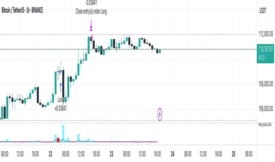
VWAP StrategyVWAP and volatility filters for structured intraday trades.
How the Strategy Works
1. VWAP Anchored to Session
VWAP is calculated from the start of each trading day.
Standard deviations are used to create bands above/below the VWAP.
2. Entry Triggers: Al Brooks H1/H2 and L1/L2
H1/H2 (Long Entry): Opens below 2nd lower deviation, closes above it.
L1/L2 (Short Entry): Opens above 2nd upper deviation, closes below it.
3. Volatility Filter (ATR)
Skips trades when deviation bands are too tight (< 3 ATRs).
4. Stop Loss
Based on the signal bar’s high/low ± stop buffer.
Longs: signalBarLow - stopBuffer
Shorts: signalBarHigh + stopBuffer
5. Take Profit / Exit Target
Exit logic is customizable per side:
VWAP, Deviation Band, or None
6. Safety Exit
Exits early if X consecutive bars go against the trade.
Longs: X red bars
Shorts: X green bars
Explanation of Strategy Inputs
- Stop Buffer: Distance from signal bar for stop-loss.
- Long/Short Exit Rule: VWAP, Deviation Band, or None
- Long/Short Target Deviation: Standard deviation for target exit.
- Enable Safety Exit: Toggle emergency exit.
- Opposing Bars: Number of opposing candles before safety exit.
- Allow Long/Short Trades: Enable or disable entry side.
- Show VWAP/Entry Bands: Toggle visual aids.
- Highlight Low Vol Zones: Orange shading for low volatility skips.
Tuning Tips
- Stop buffer: Use 1–5 points.
- Target deviation: Start with VWAP. In strong trends use 2nd deviation and turn off the counter-trend entry.
- Safety exit: 3 bars recommended.
- Disable short/long side to focus on one type of reversal.
Backtest Setup Suggestions
- initial_capital = 2000
- default_qty_value = 1 (fixed contracts or percent-of-equity)
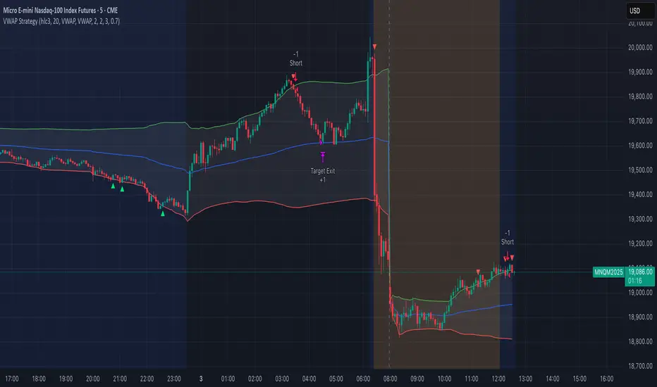
RSI + Stochastic + WMA StrategyThis script is designed for TradingView and serves as a trading strategy (not just a visual indicator). It's intended for backtesting, strategy optimization, or live trading signal generation using a combination of popular technical indicators.
📊 Indicators Used in the Strategy:
Indicator Description
RSI (Relative Strength Index) Measures momentum; identifies overbought (>70) or oversold (<30) conditions.
Stochastic Oscillator (%K & %D) Detects momentum reversal points via crossovers. Useful for timing entries.
WMA (Weighted Moving Average) Identifies the trend direction (used as a trend filter).
📈 Trading Logic / Strategy Rules:
📌 Long Entry Condition (Buy Signal):
All 3 conditions must be true:
RSI is Oversold → RSI < 30
Stochastic Crossover Upward → %K crosses above %D
Price is above WMA → Confirms uptrend direction
👉 Interpretation: Market was oversold, momentum is turning up, and price confirms uptrend — bullish entry.
📌 Short Entry Condition (Sell Signal):
All 3 conditions must be true:
RSI is Overbought → RSI > 70
Stochastic Crossover Downward → %K crosses below %D
Price is below WMA → Confirms downtrend direction
👉 Interpretation: Market is overbought, momentum is turning down, and price confirms downtrend — bearish entry.
🔄 Strategy Execution (Backtesting Logic):
The script uses:
pinescript
Copy
Edit
strategy.entry("LONG", strategy.long)
strategy.entry("SHORT", strategy.short)
These are Pine Script functions to place buy and sell orders automatically when the above conditions are met. This allows you to:
Backtest the strategy
Measure win/loss ratio, drawdown, and profitability
Optimize indicator settings using TradingView Strategy Tester
📊 Visual Aids (Charts):
Plots WMA Line: Orange line for trend direction
Overbought/Oversold Zones: Horizontal lines at 70 (red) and 30 (green) for RSI visualization
⚡ Strategy Type Summary:
Category Setting
Strategy Type Momentum Reversal + Trend Filter
Timeframe Flexible (Works best on 1H, 4H, Daily)
Trading Style Swing/Intraday
Risk Profile Medium to High (due to momentum triggers)
Uses Leverage Possible (adjust risk accordingly)
Gold Pro StrategyHere’s the strategy description in a chat format:
---
**Gold (XAU/USD) Trend-Following Strategy**
This **trend-following strategy** is designed for trading gold (XAU/USD) by combining moving averages, MACD momentum indicators, and RSI filters to capture sustained trends while managing volatility risks. The strategy uses volatility-adjusted stops to protect gains and prevent overexposure during erratic price movements. The aim is to take advantage of trending markets by confirming momentum and ensuring entries are not made at extreme levels.
---
**Key Components**
1. **Trend Identification**
- **50 vs 200 EMA Crossover**
- **Bullish Trend:** 50 EMA crosses above 200 EMA, and the price closes above the 200 EMA
- **Bearish Trend:** 50 EMA crosses below 200 EMA, and the price closes below the 200 EMA
2. **Momentum Confirmation**
- **MACD (12,26,9)**
- **Buy Signal:** MACD line crosses above the signal line
- **Sell Signal:** MACD line crosses below the signal line
- **RSI (14 Period)**
- **Bullish Zone:** RSI between 50-70 to avoid overbought conditions
- **Bearish Zone:** RSI between 30-50 to avoid oversold conditions
3. **Entry Criteria**
- **Long Entry:** Bullish trend, MACD bullish crossover, and RSI between 50-70
- **Short Entry:** Bearish trend, MACD bearish crossover, and RSI between 30-50
4. **Exit & Risk Management**
- **ATR Trailing Stops (14 Period):**
- Initial Stop: 3x ATR from entry price
- Trailing Stop: Adjusts to lock in profits as price moves favorably
- **Position Sizing:** 100% of equity per trade (high-risk strategy)
---
**Key Logic Flow**
1. **Trend Filter:** Use the 50/200 EMA relationship to define the market's direction
2. **Momentum Confirmation:** Confirm trend momentum with MACD crossovers
3. **RSI Validation:** Ensure RSI is within non-extreme ranges before entering trades
4. **Volatility-Based Risk Management:** Use ATR stops to manage market volatility
---
**Visual Cues**
- **Blue Line:** 50 EMA
- **Red Line:** 200 EMA
- **Green Triangles:** Long entry signals
- **Red Triangles:** Short entry signals
---
**Strengths**
- **Clear Trend Focus:** Avoids counter-trend trades
- **RSI Filter:** Prevents entering overbought or oversold conditions
- **ATR Stops:** Adapts to gold’s inherent volatility
- **Simple Rules:** Easy to follow with minimal inputs
---
**Weaknesses & Risks**
- **Infrequent Signals:** 50/200 EMA crossovers are rare
- **Potential Missed Opportunities:** Strict RSI criteria may miss some valid trends
- **Aggressive Position Sizing:** 100% equity allocation can lead to large drawdowns
- **No Profit Targets:** Relies on trailing stops rather than defined exit targets
---
**Performance Profile**
| Metric | Expected Range |
|----------------------|---------------------|
| Annual Trades | 4-8 |
| Win Rate | 55-65% |
| Max Drawdown | 25-35% |
| Profit Factor | 1.8-2.5 |
---
**Optimization Recommendations**
1. **Increase Trade Frequency**
Adjust the EMAs to shorter periods:
- `emaFastLen = input.int(30, "Fast EMA")`
- `emaSlowLen = input.int(150, "Slow EMA")`
2. **Relax RSI Filters**
Adjust the RSI range to:
- `rsiBullish = rsi > 45 and rsi < 75`
- `rsiBearish = rsi < 55 and rsi > 25`
3. **Add Profit Targets**
Introduce a profit target at 1.5% above entry:
```pine
strategy.exit("Long Exit", "Long",
stop=longStopPrice,
profit=close*1.015, // 1.5% target
trail_offset=trailOffset)
```
4. **Reduce Position Sizing**
Risk a smaller percentage per trade:
- `default_qty_value=25`
---
**Best Use Case**
This strategy excels in **strong trending markets** such as gold rallies during economic or geopolitical crises. However, during sideways or choppy market conditions, the strategy might require manual intervention to avoid false signals. Additionally, integrating fundamental analysis—like monitoring USD weakness or geopolitical risks—can enhance its effectiveness.
---
This strategy offers a balanced approach for trading gold, combining trend-following principles with risk management tailored to the volatility of the market.
