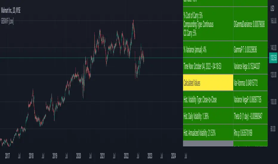
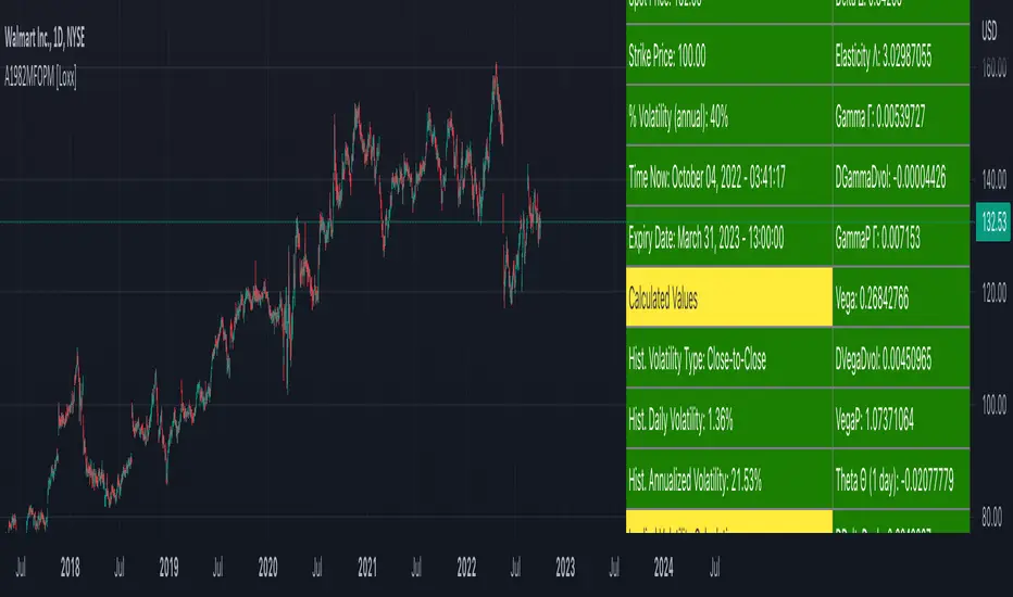
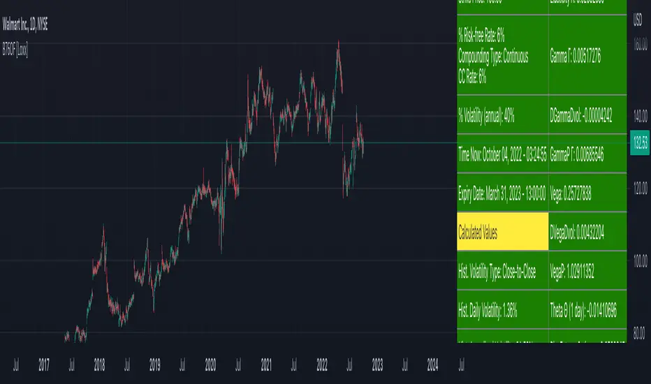
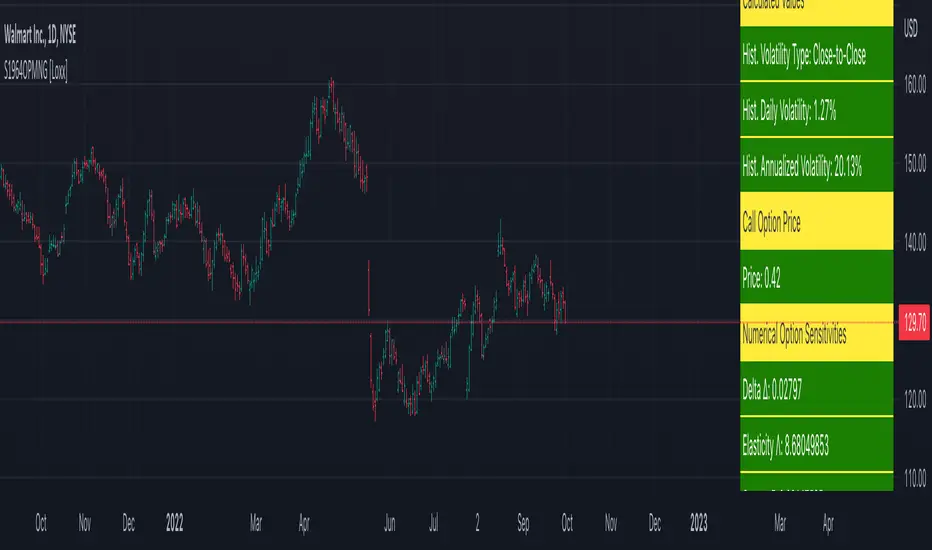
Perpetual American Options [Loxx]Perpetual American Options is Perpetual American Options pricing model. This indicator also includes numerical greeks.
American Perpetual Options
While there in general is no closed-form solution for American options (except for non-dividend-paying stock call options) it is possible to find a closed-form solution for options with an infinite time to expiration. The reason is that the time to expiration will always be the same: infinite. The time to maturity, therefore, does not depend on at what point in time we look at the valuation problem, which makes the valuation problem independent of time McKean (1965) and Merton (1973) gives closed-form solutions for American perpetual options. For a call option we have
c = (X / (y1 - 1)) * ((y1 - 1)/y1 * S/X)^y1
where
y1 = 1/2 - b/v^2 + ((b/v^2 - 1/2)^2 + 2*r/v^2)^0.5
If b >= r, then there is never optimal to exercise a call option. In the case of an American perpetual put, we have
p = X/(1-y2) * (((y2 - 1) / y2) * S/X)^y2
where
y2 = 1/2 - b/v^2 - ((b/v^2 - 1/2)^2 + 2*r/v^2)^0.5
In practice, one can naturally discuss if there is such a thing as infinite time to maturity. For instance, credit risk could play an important role: Even when you are buying an option from an AAA bank, there is no guarantee the bank will be around forever.
b=r options on non-dividend paying stock
b=r-q options on stock or index paying a dividend yield of q
b=0 options on futures
b=r-rf currency options (where rf is the rate in the second currency)
Inputs
S = Stock price.
K = Strike price of option.
T = Time to expiration in years.
r = Risk-free rate
c = Cost of Carry
V = Variance of the underlying asset price
cnd1(x) = Cumulative Normal Distribution
cbnd3(x) = Cumulative Bivariate Normal Distribution
nd(x) = Standard Normal Density Function
convertingToCCRate(r, cmp ) = Rate compounder
Numerical Greeks or Greeks by Finite Difference
Analytical Greeks are the standard approach to estimating Delta, Gamma etc... That is what we typically use when we can derive from closed form solutions. Normally, these are well-defined and available in text books. Previously, we relied on closed form solutions for the call or put formulae differentiated with respect to the Black Scholes parameters. When Greeks formulae are difficult to develop or tease out, we can alternatively employ numerical Greeks - sometimes referred to finite difference approximations. A key advantage of numerical Greeks relates to their estimation independent of deriving mathematical Greeks. This could be important when we examine American options where there may not technically exist an exact closed form solution that is straightforward to work with. (via VinegarHill FinanceLabs)
Things to know
Only works on the daily timeframe and for the current source price.
You can adjust the text size to fit the screen
Tìm kiếm tập lệnh với "通达信+选股公式+换手率+0.5+源码"
[blackcat] L3 Candle Skew 3821 TraderLevel 3
Background
By modeling skew to produce long and short entry points.
Function
The concept of skew comes from physics and statistics, and is used in market technical analysis to reflect the expectation of future stock price distribution. Because the return distribution of stocks in the trend market has skew (Skew), it is reasonable to judge the trend continuity according to the historical and current skew. It is precisely because the stock price rises that there is a skew. The greater the strength of the rise, the greater the angle of inclination and the greater the skew. The degree of this upward or downward slope in the statistical distribution of stock prices is defined as skew. Through the size of skew, we can know the direction, inertia and extent of the stock's rise or fall, and find stocks with a high probability of quick profit. The technical indicator introduced today is a simplified but effective stock price skew model used to generate buying and selling points.
The principle of this technical indicator is based on the success rate test results of different moving averages corresponding to different skews as follows:
10 trading cycles profit 5% success rate (%)
5 period moving average 10 period moving average 20 period moving average 30 period moving average 60 period moving average
skew>=0 51.36 52.26 52.65 52.55 52.08
skew>=0.5 55.44 58.06 60.56 62.37 65.66
skew>=1 59.72 63.06 67.07 69.78 70.62
skew>=1.5 63.01 67.08 71.61 72.9 70.61
skew>=2 65.53 70.22 74.18 73.76 70.12
skew>=2.5 67.89 72.93 75.32 73.66 68.92
skew>=3 70.07 75.32 75.69 72.54 67.45
skew>=3.5 71.85 77.05 75.32 73.63 63.82
skew>=4 73.6 78.06 74.19 68.96 59.91
skew>=4.5 76.04 78.56 72.85 69.55 49.24
skew>=5 77.44 78.88 71.58 67.28 51.69
skew>=5.5 78.97 78.39 70.33 64.31 49.7
skew>=6 79.68 78.07 68.82 61.65 53.57
Table 1
As can be seen from the above table, with the increase of the 5-period and 10-period moving average skew values, the success rate is increasing, but after the 20- and 30-period moving average skew values increase to an upper bound, it shows a downward trend. When the skew of the 20-period and 30-period moving averages is greater than 0.5, the 10-period profit of 5% is above 60%, and when it is greater than 1.5, the success rate can reach above 70%. The larger the 5-period moving average skew, the higher the success rate, but often because the short-term skew is too large, the stock price has risen rapidly to a high level, and chasing up is risky, which is not suitable for the investment habits of most people, so prudent investors may like to do swings. Investors may wish to pay more attention to the skew of the 20-period and 30-period moving averages. Based on the above analysis, as a short-term trading enthusiast, I need to choose the 5-period and 10-period moving average skew, and consider the medium-term trend as a compromise, and I also need to consider the 20-period moving average skew. Finally, according to the principle of personal preference, I chose 3 groups of periods based on Fibonacci magic numbers: 3 periods, 8 periods, 21 periods, and skews that take into account both short-term and mid-line trends. So, I named this indicator number 3821 as a distinction.
002084 1D from TradingView
BTCUSDT 1H from TradingView
Tesla 1D from TradingView
Samuelson 1965 Option Pricing Formula [Loxx]Samuelson 1965 Option Pricing Formula is an options pricing formula that pre-dates Black-Scholes-Merton. This version includes Analytical Greeks.
Samuelson (1965; see also Smith, 1976) assumed the asset price follows a geometric Brownian motion with positive drift, p. In this way he allowed for positive interest rates and a risk premium.
c = SN(d1) * e^((rho - omega) * T) - Xe^(-omega * T)N(d2)
d1 = (log(S / X) + (rho + v^2 / 2) * T) / (v * T^0.5)
d2 = d1 - (v * T^0.5)
where rho is the average rate of growth of the share price and omega is the average rate of growth in the value of the call. This is different from the Boness model in that the Samuelson model can take into account that the expected return from the option is larger than that of the underlying asset omega > rho.
Analytical Greeks
Delta Greeks: Delta, DDeltaDvol, Elasticity
Gamma Greeks: Gamma, GammaP, DGammaDvol, Speed
Vega Greeks: Vega , DVegaDvol/Vomma, VegaP
Theta Greeks: Theta
Rate/Carry Greeks: Option growth rate sensitivity, Share growth rate sensitivity
Probability Greeks: StrikeDelta, Risk Neutral Density
Inputs
S = Stock price.
X = Strike price of option.
T = Time to expiration in years.
omega = Average growth rate option
rho = Average growth rate share
v = Volatility of the underlying asset price
cnd (x) = The cumulative normal distribution function
nd(x) = The standard normal density function
convertingToCCRate(r, cmp ) = Rate compounder
Things to know
Only works on the daily timeframe and for the current source price.
You can adjust the text size to fit the screen

Boness 1964 Option Pricing Formula [Loxx]Boness 1964 Option Pricing Formula is an options pricing model that pre-dates Black-Scholes-Merton. This model includes Analytical Greeks.
Boness (1964) assumed a lognormal asset price. Boness derives the following value for a call option:
c = SN(d1) - Xe^(rho * T)N(d2)
d1 = (log(S / X) + (rho + v^2 / 2) * T) / (v * T^0.5)
d2 = d1 - (v * T^0.5)
where rho is the expected rate of return to the asset.
Analytical Greeks
Delta Greeks: Delta, DDeltaDvol, Elasticity
Gamma Greeks: Gamma, GammaP, DGammaDvol, Speed
Vega Greeks: Vega , DVegaDvol/Vomma, VegaP
Theta Greeks: Theta
Probability Greeks: StrikeDelta, Risk Neutral Density, Rho Expected Rate of Return
Inputs
S = Stock price.
X = Strike price of option.
T = Time to expiration in years.
r = Expected Rate of Return
v = Volatility of the underlying asset price
cnd (x) = The cumulative normal distribution function
nd(x) = The standard normal density function
convertingToCCRate(r, cmp ) = Rate compounder
Things to know
Only works on the daily timeframe and for the current source price.
You can adjust the text size to fit the screen
Generalized Black-Scholes-Merton on Variance Form [Loxx]Generalized Black-Scholes-Merton on Variance Form is an adaptation of the Black-Scholes-Merton Option Pricing Model including Numerical Greeks. The following information is an excerpt from Espen Gaarder Haug's book "Option Pricing Formulas". This version is to price Options using variance instead of volatility.
Black- Scholes- Merton on Variance Form
In some circumstances, it is useful to rewrite the BSM formula using variance as input instead of volatility, V = v^2:
c = S * e^((b - r) * T) * N(d1) - X * e^(-r * T) * N(d2)
p = X * e^(-r * T) * N(-d2) - S * e^((b - r) * T) * N(-d1)
where
d1 = (log(S / X) + (b + V^2 / 2) * T) / (V * T)^0.5
d2 = d1 - (V * T)^0.5
BSM on variance form clearly gives the same price as when written on volatility form. The variance form is used indirectly in terms of its partial derivatives in some stochastic variance models, as well as for hedging of variance swaps. The BSM on variance form moreover admits an interesting symmetry between put and call options as discussed by Adamchuk and Haug (2005) at www.wilmott.com .
c(S, X, T, r, b, V) = -c(-S, -X, -T, -r, -b, -V)
and
p(S, X, T, r, b, V) = -p(-S, -X, -T, -r, -b, -V)
It is possible to find several similar symmetries if we introduce imaginary numbers.
b = r ... gives the Black and Scholes (1973) stock option model.
b = r — q ... gives the Merton (1973) stock option model with continuous dividend yield q.
b = 0 ... gives the Black (1976) futures option model.
b = 0 and r = 0 ... gives the Asay (1982) margined futures option model.
b = r — rf ... gives the Garman and Kohlhagen (1983) currency option model.
Inputs
S = Stock price.
X = Strike price of option.
T = Time to expiration in years.
r = Risk-free rate
cc = Cost of Carry
V = Variance of the underlying asset price
cnd (x) = The cumulative normal distribution function
nd(x) = The standard normal density function
convertingToCCRate(r, cmp ) = Rate compounder
Numerical Greeks or Greeks by Finite Difference
Analytical Greeks are the standard approach to estimating Delta, Gamma etc... That is what we typically use when we can derive from closed form solutions. Normally, these are well-defined and available in text books. Previously, we relied on closed form solutions for the call or put formulae differentiated with respect to the Black Scholes parameters. When Greeks formulae are difficult to develop or tease out, we can alternatively employ numerical Greeks - sometimes referred to finite difference approximations. A key advantage of numerical Greeks relates to their estimation independent of deriving mathematical Greeks. This could be important when we examine American options where there may not technically exist an exact closed form solution that is straightforward to work with. (via VinegarHill FinanceLabs)
Things to know
Only works on the daily timeframe and for the current source price.
You can adjust the text size to fit the screen
Asay (1982) Margined Futures Option Pricing Model [Loxx]Asay (1982) Margined Futures Option Pricing Model is an adaptation of the Black-Scholes-Merton Option Pricing Model including Analytical Greeks and implied volatility calculations. The following information is an excerpt from Espen Gaarder Haug's book "Option Pricing Formulas". This version is to price Options on Futures where premium is fully margined. This means the Risk-free Rate, dividend, and cost to carry are all zero. The options sensitivities (Greeks) are the partial derivatives of the Black-Scholes-Merton ( BSM ) formula. Analytical Greeks for our purposes here are broken down into various categories:
Delta Greeks: Delta, DDeltaDvol, Elasticity
Gamma Greeks: Gamma, GammaP, DGammaDvol, Speed
Vega Greeks: Vega , DVegaDvol/Vomma, VegaP
Theta Greeks: Theta
Probability Greeks: StrikeDelta, Risk Neutral Density
(See the code for more details)
Black-Scholes-Merton Option Pricing
The Black-Scholes-Merton model can be "generalized" by incorporating a cost-of-carry rate b. This model can be used to price European options on stocks, stocks paying a continuous dividend yield, options on futures , and currency options:
c = S * e^((b - r) * T) * N(d1) - X * e^(-r * T) * N(d2)
p = X * e^(-r * T) * N(-d2) - S * e^((b - r) * T) * N(-d1)
where
d1 = (log(S / X) + (b + v^2 / 2) * T) / (v * T^0.5)
d2 = d1 - v * T^0.5
b = r ... gives the Black and Scholes (1973) stock option model.
b = r — q ... gives the Merton (1973) stock option model with continuous dividend yield q.
b = 0 ... gives the Black (1976) futures option model.
b = 0 and r = 0 ... gives the Asay (1982) margined futures option model. <== this is the one used for this indicator!
b = r — rf ... gives the Garman and Kohlhagen (1983) currency option model.
Inputs
S = Stock price.
X = Strike price of option.
T = Time to expiration in years.
r = Risk-free rate
d = dividend yield
v = Volatility of the underlying asset price
cnd (x) = The cumulative normal distribution function
nd(x) = The standard normal density function
convertingToCCRate(r, cmp ) = Rate compounder
gImpliedVolatilityNR(string CallPutFlag, float S, float x, float T, float r, float b, float cm , float epsilon) = Implied volatility via Newton Raphson
gBlackScholesImpVolBisection(string CallPutFlag, float S, float x, float T, float r, float b, float cm ) = implied volatility via bisection
Implied Volatility: The Bisection Method
The Newton-Raphson method requires knowledge of the partial derivative of the option pricing formula with respect to volatility ( vega ) when searching for the implied volatility . For some options (exotic and American options in particular), vega is not known analytically. The bisection method is an even simpler method to estimate implied volatility when vega is unknown. The bisection method requires two initial volatility estimates (seed values):
1. A "low" estimate of the implied volatility , al, corresponding to an option value, CL
2. A "high" volatility estimate, aH, corresponding to an option value, CH
The option market price, Cm , lies between CL and cH . The bisection estimate is given as the linear interpolation between the two estimates:
v(i + 1) = v(L) + (c(m) - c(L)) * (v(H) - v(L)) / (c(H) - c(L))
Replace v(L) with v(i + 1) if c(v(i + 1)) < c(m), or else replace v(H) with v(i + 1) if c(v(i + 1)) > c(m) until |c(m) - c(v(i + 1))| <= E, at which point v(i + 1) is the implied volatility and E is the desired degree of accuracy.
Implied Volatility: Newton-Raphson Method
The Newton-Raphson method is an efficient way to find the implied volatility of an option contract. It is nothing more than a simple iteration technique for solving one-dimensional nonlinear equations (any introductory textbook in calculus will offer an intuitive explanation). The method seldom uses more than two to three iterations before it converges to the implied volatility . Let
v(i + 1) = v(i) + (c(v(i)) - c(m)) / (dc / dv (i))
until |c(m) - c(v(i + 1))| <= E at which point v(i + 1) is the implied volatility , E is the desired degree of accuracy, c(m) is the market price of the option, and dc/ dv (i) is the vega of the option evaluaated at v(i) (the sensitivity of the option value for a small change in volatility ).
Things to know
Only works on the daily timeframe and for the current source price.
You can adjust the text size to fit the screen
Black-76 Options on Futures [Loxx]Black-76 Options on Futures is an adaptation of the Black-Scholes-Merton Option Pricing Model including Analytical Greeks and implied volatility calculations. The following information is an excerpt from Espen Gaarder Haug's book "Option Pricing Formulas". This version is to price Options on Futures. The options sensitivities (Greeks) are the partial derivatives of the Black-Scholes-Merton ( BSM ) formula. Analytical Greeks for our purposes here are broken down into various categories:
Delta Greeks: Delta, DDeltaDvol, Elasticity
Gamma Greeks: Gamma, GammaP, DGammaDvol, Speed
Vega Greeks: Vega , DVegaDvol/Vomma, VegaP
Theta Greeks: Theta
Rate/Carry Greeks: Rho futures option
Probability Greeks: StrikeDelta, Risk Neutral Density
(See the code for more details)
Black-Scholes-Merton Option Pricing
The Black-Scholes-Merton model can be "generalized" by incorporating a cost-of-carry rate b. This model can be used to price European options on stocks, stocks paying a continuous dividend yield, options on futures , and currency options:
c = S * e^((b - r) * T) * N(d1) - X * e^(-r * T) * N(d2)
p = X * e^(-r * T) * N(-d2) - S * e^((b - r) * T) * N(-d1)
where
d1 = (log(S / X) + (b + v^2 / 2) * T) / (v * T^0.5)
d2 = d1 - v * T^0.5
b = r ... gives the Black and Scholes (1973) stock option model.
b = r — q ... gives the Merton (1973) stock option model with continuous dividend yield q.
b = 0 ... gives the Black (1976) futures option model. <== this is the one used for this indicator!
b = 0 and r = 0 ... gives the Asay (1982) margined futures option model.
b = r — rf ... gives the Garman and Kohlhagen (1983) currency option model.
Inputs
S = Stock price.
X = Strike price of option.
T = Time to expiration in years.
r = Risk-free rate
d = dividend yield
v = Volatility of the underlying asset price
cnd (x) = The cumulative normal distribution function
nd(x) = The standard normal density function
convertingToCCRate(r, cmp ) = Rate compounder
gImpliedVolatilityNR(string CallPutFlag, float S, float x, float T, float r, float b, float cm , float epsilon) = Implied volatility via Newton Raphson
gBlackScholesImpVolBisection(string CallPutFlag, float S, float x, float T, float r, float b, float cm ) = implied volatility via bisection
Implied Volatility: The Bisection Method
The Newton-Raphson method requires knowledge of the partial derivative of the option pricing formula with respect to volatility ( vega ) when searching for the implied volatility . For some options (exotic and American options in particular), vega is not known analytically. The bisection method is an even simpler method to estimate implied volatility when vega is unknown. The bisection method requires two initial volatility estimates (seed values):
1. A "low" estimate of the implied volatility , al, corresponding to an option value, CL
2. A "high" volatility estimate, aH, corresponding to an option value, CH
The option market price, Cm , lies between CL and cH . The bisection estimate is given as the linear interpolation between the two estimates:
v(i + 1) = v(L) + (c(m) - c(L)) * (v(H) - v(L)) / (c(H) - c(L))
Replace v(L) with v(i + 1) if c(v(i + 1)) < c(m), or else replace v(H) with v(i + 1) if c(v(i + 1)) > c(m) until |c(m) - c(v(i + 1))| <= E, at which point v(i + 1) is the implied volatility and E is the desired degree of accuracy.
Implied Volatility: Newton-Raphson Method
The Newton-Raphson method is an efficient way to find the implied volatility of an option contract. It is nothing more than a simple iteration technique for solving one-dimensional nonlinear equations (any introductory textbook in calculus will offer an intuitive explanation). The method seldom uses more than two to three iterations before it converges to the implied volatility . Let
v(i + 1) = v(i) + (c(v(i)) - c(m)) / (dc / dv (i))
until |c(m) - c(v(i + 1))| <= E at which point v(i + 1) is the implied volatility , E is the desired degree of accuracy, c(m) is the market price of the option, and dc/ dv (i) is the vega of the option evaluaated at v(i) (the sensitivity of the option value for a small change in volatility ).
Things to know
Only works on the daily timeframe and for the current source price.
You can adjust the text size to fit the screen
Garman and Kohlhagen (1983) for Currency Options [Loxx]Garman and Kohlhagen (1983) for Currency Options is an adaptation of the Black-Scholes-Merton Option Pricing Model including Analytical Greeks and implied volatility calculations. The following information is an excerpt from Espen Gaarder Haug's book "Option Pricing Formulas". This version of BSMOPM is to price Currency Options. The options sensitivities (Greeks) are the partial derivatives of the Black-Scholes-Merton ( BSM ) formula. Analytical Greeks for our purposes here are broken down into various categories:
Delta Greeks: Delta, DDeltaDvol, Elasticity
Gamma Greeks: Gamma, GammaP, DGammaDSpot/speed, DGammaDvol/Zomma
Vega Greeks: Vega , DVegaDvol/Vomma, VegaP, Speed
Theta Greeks: Theta
Rate/Carry Greeks: Rho, Rho futures option, Carry Rho, Phi/Rho2
Probability Greeks: StrikeDelta, Risk Neutral Density
(See the code for more details)
Black-Scholes-Merton Option Pricing for Currency Options
The Garman and Kohlhagen (1983) modified Black-Scholes model can be used to price European currency options; see also Grabbe (1983). The model is mathematically equivalent to the Merton (1973) model presented earlier. The only difference is that the dividend yield is replaced by the risk-free rate of the foreign currency rf:
c = S * e^(-rf * T) * N(d1) - X * e^(-r * T) * N(d2)
p = X * e^(-r * T) * N(-d2) - S * e^(-rf * T) * N(-d1)
where
d1 = (log(S / X) + (r - rf + v^2 / 2) * T) / (v * T^0.5)
d2 = d1 - v * T^0.5
For more information on currency options, see DeRosa (2000)
Inputs
S = Stock price.
X = Strike price of option.
T = Time to expiration in years.
r = Risk-free rate
rf = Risk-free rate of the foreign currency
v = Volatility of the underlying asset price
cnd (x) = The cumulative normal distribution function
nd(x) = The standard normal density function
convertingToCCRate(r, cmp ) = Rate compounder
gImpliedVolatilityNR(string CallPutFlag, float S, float x, float T, float r, float b, float cm , float epsilon) = Implied volatility via Newton Raphson
gBlackScholesImpVolBisection(string CallPutFlag, float S, float x, float T, float r, float b, float cm ) = implied volatility via bisection
Implied Volatility: The Bisection Method
The Newton-Raphson method requires knowledge of the partial derivative of the option pricing formula with respect to volatility ( vega ) when searching for the implied volatility . For some options (exotic and American options in particular), vega is not known analytically. The bisection method is an even simpler method to estimate implied volatility when vega is unknown. The bisection method requires two initial volatility estimates (seed values):
1. A "low" estimate of the implied volatility , al, corresponding to an option value, CL
2. A "high" volatility estimate, aH, corresponding to an option value, CH
The option market price, Cm , lies between CL and cH . The bisection estimate is given as the linear interpolation between the two estimates:
v(i + 1) = v(L) + (c(m) - c(L)) * (v(H) - v(L)) / (c(H) - c(L))
Replace v(L) with v(i + 1) if c(v(i + 1)) < c(m), or else replace v(H) with v(i + 1) if c(v(i + 1)) > c(m) until |c(m) - c(v(i + 1))| <= E, at which point v(i + 1) is the implied volatility and E is the desired degree of accuracy.
Implied Volatility: Newton-Raphson Method
The Newton-Raphson method is an efficient way to find the implied volatility of an option contract. It is nothing more than a simple iteration technique for solving one-dimensional nonlinear equations (any introductory textbook in calculus will offer an intuitive explanation). The method seldom uses more than two to three iterations before it converges to the implied volatility . Let
v(i + 1) = v(i) + (c(v(i)) - c(m)) / (dc / dv (i))
until |c(m) - c(v(i + 1))| <= E at which point v(i + 1) is the implied volatility , E is the desired degree of accuracy, c(m) is the market price of the option, and dc/ dv (i) is the vega of the option evaluaated at v(i) (the sensitivity of the option value for a small change in volatility ).
Things to know
Only works on the daily timeframe and for the current source price.
You can adjust the text size to fit the screen
Related indicators:
BSM OPM 1973 w/ Continuous Dividend Yield
Black-Scholes 1973 OPM on Non-Dividend Paying Stocks
Generalized Black-Scholes-Merton w/ Analytical Greeks
Generalized Black-Scholes-Merton Option Pricing Formula
Sprenkle 1964 Option Pricing Model w/ Num. Greeks
Modified Bachelier Option Pricing Model w/ Num. Greeks
Bachelier 1900 Option Pricing Model w/ Numerical Greeks

BSM OPM 1973 w/ Continuous Dividend Yield [Loxx]Generalized Black-Scholes-Merton w/ Analytical Greeks is an adaptation of the Black-Scholes-Merton Option Pricing Model including Analytical Greeks and implied volatility calculations. The following information is an excerpt from Espen Gaarder Haug's book "Option Pricing Formulas". The options sensitivities (Greeks) are the partial derivatives of the Black-Scholes-Merton ( BSM ) formula. Analytical Greeks for our purposes here are broken down into various categories:
Delta Greeks: Delta, DDeltaDvol, Elasticity
Gamma Greeks: Gamma, GammaP, DGammaDSpot/speed, DGammaDvol/Zomma
Vega Greeks: Vega , DVegaDvol/Vomma, VegaP
Theta Greeks: Theta
Rate/Carry Greeks: Rho, Rho futures option, Carry Rho, Phi/Rho2
Probability Greeks: StrikeDelta, Risk Neutral Density
(See the code for more details)
Black-Scholes-Merton Option Pricing
The Black-Scholes-Merton model can be "generalized" by incorporating a cost-of-carry rate b. This model can be used to price European options on stocks, stocks paying a continuous dividend yield, options on futures, and currency options:
c = S * e^((b - r) * T) * N(d1) - X * e^(-r * T) * N(d2)
p = X * e^(-r * T) * N(-d2) - S * e^((b - r) * T) * N(-d1)
where
d1 = (log(S / X) + (b + v^2 / 2) * T) / (v * T^0.5)
d2 = d1 - v * T^0.5
b = r ... gives the Black and Scholes (1973) stock option model.
b = r — q ... gives the Merton (1973) stock option model with continuous dividend yield q. <== this is the one used for this indicator!
b = 0 ... gives the Black (1976) futures option model.
b = 0 and r = 0 ... gives the Asay (1982) margined futures option model.
b = r — rf ... gives the Garman and Kohlhagen (1983) currency option model.
Inputs
S = Stock price.
X = Strike price of option.
T = Time to expiration in years.
r = Risk-free rate
d = dividend yield
v = Volatility of the underlying asset price
cnd (x) = The cumulative normal distribution function
nd(x) = The standard normal density function
convertingToCCRate(r, cmp ) = Rate compounder
gImpliedVolatilityNR(string CallPutFlag, float S, float x, float T, float r, float b, float cm , float epsilon) = Implied volatility via Newton Raphson
gBlackScholesImpVolBisection(string CallPutFlag, float S, float x, float T, float r, float b, float cm ) = implied volatility via bisection
Implied Volatility: The Bisection Method
The Newton-Raphson method requires knowledge of the partial derivative of the option pricing formula with respect to volatility ( vega ) when searching for the implied volatility . For some options (exotic and American options in particular), vega is not known analytically. The bisection method is an even simpler method to estimate implied volatility when vega is unknown. The bisection method requires two initial volatility estimates (seed values):
1. A "low" estimate of the implied volatility , al, corresponding to an option value, CL
2. A "high" volatility estimate, aH, corresponding to an option value, CH
The option market price, Cm , lies between CL and cH . The bisection estimate is given as the linear interpolation between the two estimates:
v(i + 1) = v(L) + (c(m) - c(L)) * (v(H) - v(L)) / (c(H) - c(L))
Replace v(L) with v(i + 1) if c(v(i + 1)) < c(m), or else replace v(H) with v(i + 1) if c(v(i + 1)) > c(m) until |c(m) - c(v(i + 1))| <= E, at which point v(i + 1) is the implied volatility and E is the desired degree of accuracy.
Implied Volatility: Newton-Raphson Method
The Newton-Raphson method is an efficient way to find the implied volatility of an option contract. It is nothing more than a simple iteration technique for solving one-dimensional nonlinear equations (any introductory textbook in calculus will offer an intuitive explanation). The method seldom uses more than two to three iterations before it converges to the implied volatility . Let
v(i + 1) = v(i) + (c(v(i)) - c(m)) / (dc / dv (i))
until |c(m) - c(v(i + 1))| <= E at which point v(i + 1) is the implied volatility , E is the desired degree of accuracy, c(m) is the market price of the option, and dc/ dv (i) is the vega of the option evaluaated at v(i) (the sensitivity of the option value for a small change in volatility ).
Things to know
Only works on the daily timeframe and for the current source price.
You can adjust the text size to fit the screen

Sprenkle 1964 Option Pricing Model w/ Num. Greeks [Loxx]Sprenkle 1964 Option Pricing Model w/ Num. Greeks is an adaptation of the Sprenkle 1964 Option Pricing Model in Pine Script. The following information is an except from Espen Gaarder Haug's book "Option Pricing Formulas".
The Sprenkle Model
Sprenkle (1964) assumed the stock price was log-normally distributed and thus that the asset price followed a geometric Brownian motion, just as in the Black and Scholes (1973) analysis. In this way he ruled out the possibility of negative stock prices, consistent with limited liability. Sprenkle moreover allowed for a drift in the asset price, thus allowing positive interest rates and risk aversion (Smith, 1976). Sprenkle assumed today's value was equal to the expected value at maturity.
c = S * e^(rho*T) * N(d1) - (1 - k) * X * N(d2)
d1 = (log(S/X) + (rho + v^2 / 2) * T) / (v * T^0.5)
d2 = d1 - (v * T^0.5)
Inputs
S = Stock price.
X = Strike price of option.
T = Time to expiration in years.
r = Risk-free rate
v = Volatility of the underlying asset price
k = Market risk aversion adjustment
rho = Average growth rate share
cnd (x) = The cumulative normal distribution function
nd(x) = The standard normal density function
nd(x) = The standard normal density function
convertingToCCRate(r, cmp) = Rate compounder
Numerical Greeks or Greeks by Finite Difference
Analytical Greeks are the standard approach to estimating Delta, Gamma etc... That is what we typically use when we can derive from closed form solutions. Normally, these are well-defined and available in text books. Previously, we relied on closed form solutions for the call or put formulae differentiated with respect to the Black Scholes parameters. When Greeks formulae are difficult to develop or tease out, we can alternatively employ numerical Greeks - sometimes referred to finite difference approximations. A key advantage of numerical Greeks relates to their estimation independent of deriving mathematical Greeks. This could be important when we examine American options where there may not technically exist an exact closed form solution that is straightforward to work with. (via VinegarHill FinanceLabs)
Things to know
Only works on the daily timeframe and for the current source price.
You can adjust the text size to fit the screen
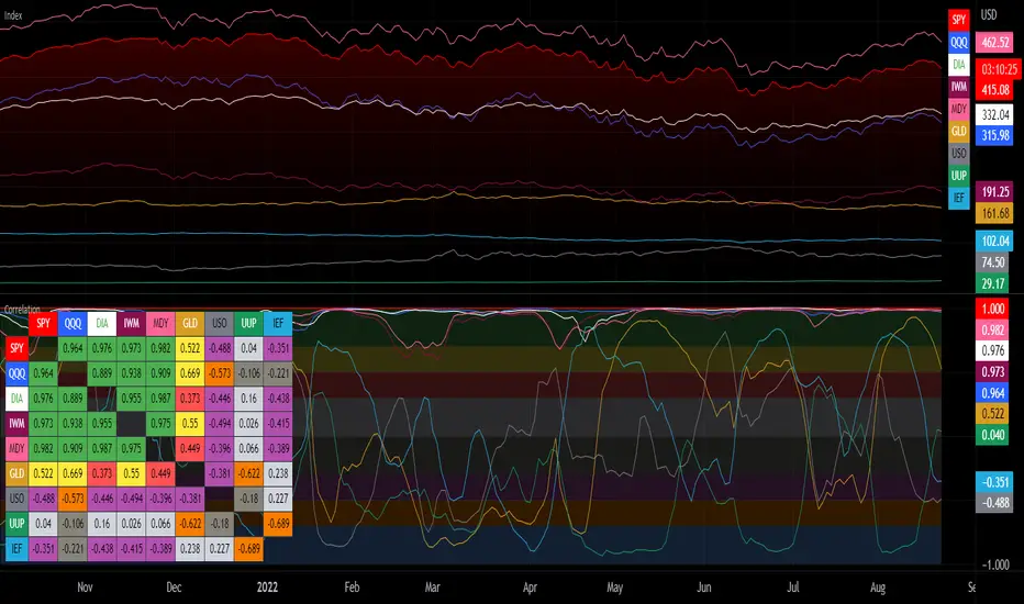
Correlation with Matrix TableCorrelation coefficient is a measure of the strength of the relationship between two values. It can be useful for market analysis, cryptocurrencies, forex and much more.
Since it "describes the degree to which two series tend to deviate from their moving average values" (1), first of all you have to set the length of these moving averages. You can also retrieve the values from another timeframe, and choose whether or not to ignore the gaps.
After selecting the reference ticker, which is not dependent from the chart you are on, you can choose up to eight other tickers to relate to it. The provided matrix table will then give you a deeper insight through all of the correlations between the chosen symbols.
Correlation values are scored on a scale from 1 to -1
A value of 1 means the correlation between the values is perfect.
A value of 0 means that there is no correlation at all.
A value of -1 indicates that the correlation is perfectly opposite.
For a better view at a glance, eight level colors are available and it is possible to modify them at will. You can even change level ranges by setting their threshold values. The background color of the matrix's cells will change accordingly to all of these choices.
The default threshold values, commonly used in statistics, are as follows:
None to weak correlation: 0 - 0.3
Weak to moderate correlation: 0.3 - 0.5
Moderate to high correlation: 0.5 - 0.7
High to perfect correlation: 0.7 - 1
Remember to be careful about spurious correlations, which are strong correlations without a real causal relationship.
(1) www.tradingview.com
Hodrick-Prescott Extrapolation of Price [Loxx]Hodrick-Prescott Extrapolation of Price is a Hodrick-Prescott filter used to extrapolate price.
The distinctive feature of the Hodrick-Prescott filter is that it does not delay. It is calculated by minimizing the objective function.
F = Sum((y(i) - x(i))^2,i=0..n-1) + lambda*Sum((y(i+1)+y(i-1)-2*y(i))^2,i=1..n-2)
where x() - prices, y() - filter values.
If the Hodrick-Prescott filter sees the future, then what future values does it suggest? To answer this question, we should find the digital low-frequency filter with the frequency parameter similar to the Hodrick-Prescott filter's one but with the values calculated directly using the past values of the "twin filter" itself, i.e.
y(i) = Sum(a(k)*x(i-k),k=0..nx-1) - FIR filter
or
y(i) = Sum(a(k)*x(i-k),k=0..nx-1) + Sum(b(k)*y(i-k),k=1..ny) - IIR filter
It is better to select the "twin filter" having the frequency-independent delay Тdel (constant group delay). IIR filters are not suitable. For FIR filters, the condition for a frequency-independent delay is as follows:
a(i) = +/-a(nx-1-i), i = 0..nx-1
The simplest FIR filter with constant delay is Simple Moving Average (SMA):
y(i) = Sum(x(i-k),k=0..nx-1)/nx
In case nx is an odd number, Тdel = (nx-1)/2. If we shift the values of SMA filter to the past by the amount of bars equal to Тdel, SMA values coincide with the Hodrick-Prescott filter ones. The exact math cannot be achieved due to the significant differences in the frequency parameters of the two filters.
To achieve the closest match between the filter values, I recommend their channel widths to be similar (for example, -6dB). The Hodrick-Prescott filter's channel width of -6dB is calculated as follows:
wc = 2*arcsin(0.5/lambda^0.25).
The channel width of -6dB for the SMA filter is calculated by numerical computing via the following equation:
|H(w)| = sin(nx*wc/2)/sin(wc/2)/nx = 0.5
Prediction algorithms:
The indicator features the two prediction methods:
Metod 1:
1. Set SMA length to 3 and shift it to the past by 1 bar. With such a length, the shifted SMA does not exist only for the last bar (Bar = 0), since it needs the value of the next future price Close(-1).
2. Calculate SMA filer's channel width. Equal it to the Hodrick-Prescott filter's one. Find lambda.
3. Calculate Hodrick-Prescott filter value at the last bar HP(0) and assume that SMA(0) with unknown Close(-1) gives the same value.
4. Find Close(-1) = 3*HP(0) - Close(0) - Close(1)
5. Increase the length of SMA to 5. Repeat all calculations and find Close(-2) = 5*HP(0) - Close(-1) - Close(0) - Close(1) - Close(2). Continue till the specified amount of future FutBars prices is calculated.
Method 2:
1. Set SMA length equal to 2*FutBars+1 and shift SMA to the past by FutBars
2. Calculate SMA filer's channel width. Equal it to the Hodrick-Prescott filter's one. Find lambda.
3. Calculate Hodrick-Prescott filter values at the last FutBars and assume that SMA behaves similarly when new prices appear.
4. Find Close(-1) = (2*FutBars+1)*HP(FutBars-1) - Sum(Close(i),i=0..2*FutBars-1), Close(-2) = (2*FutBars+1)*HP(FutBars-2) - Sum(Close(i),i=-1..2*FutBars-2), etc.
The indicator features the following inputs:
Method - prediction method
Last Bar - number of the last bar to check predictions on the existing prices (LastBar >= 0)
Past Bars - amount of previous bars the Hodrick-Prescott filter is calculated for (the more, the better, or at least PastBars>2*FutBars)
Future Bars - amount of predicted future values
The second method is more accurate but often has large spikes of the first predicted price. For our purposes here, this price has been filtered from being displayed in the chart. This is why method two starts its prediction 2 bars later than method 1. The described prediction method can be improved by searching for the FIR filter with the frequency parameter closer to the Hodrick-Prescott filter. For example, you may try Hanning, Blackman, Kaiser, and other filters with constant delay instead of SMA.
Related indicators
Itakura-Saito Autoregressive Extrapolation of Price
Helme-Nikias Weighted Burg AR-SE Extra. of Price
Weighted Burg AR Spectral Estimate Extrapolation of Price
Levinson-Durbin Autocorrelation Extrapolation of Price
Fourier Extrapolator of Price w/ Projection Forecast

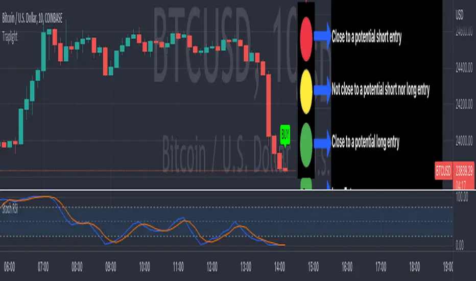
TrapLightTrap Light is built off the stochastic RSI to provide convenience and make your entries while scalping either long/short more straightforward.
Notes/Disclaimer:
This indicator is not guaranteed to work every time. Use it at your own discretion and perform your own due diligence. None of this is financial advice.
The main idea behind this is that when the stochastic RSI reaches such extremes that it often moves in a favorable direction.
K = momentum or the blue line of the stochastic RSI indicator.
Perks:
Don't have to look away from candlesticks and measure stochastic RSI's K level.
Simple visual indication of what to do.
Don't have to stare at your chart all day waiting for things to get exciting.
How to Use:
(Above the current candlestick on any timeframe)
1. When K is greater than or equal to 99.5, it shows a sell signal. This is to indicate a short entry.
2. When K is less than or equal to 0.5, it shows a buy signal. This is to indicate a long entry.
3. If neither the conditions for a short/long entry are present, it shows a circle that is like a traffic light.
Red Light: When K is between 99.5 and 95, a red circle is shown to indicate that a short entry may be available soon.
Yellow Light: When K is between 95 and 5, a yellow circle is shown to indicate that neither a long nor short entry may be available soon.
Green Light: When K is between 5 and 0.5, a green circle is shown to indicate that a long entry may be available soon.
Alerts:
Set an alert on the ticker you trade to notify you when either the green or red light is present so that you have time to prepare to make an entry either long/short.
The Code:
The PineScript is open-source and annotated to explain different parts of the script for ease of understanding.
@Credit to Kingson1 for this strategy and his feedback on its creation/implementation.
Grid Settings & MMThis script is designed to help you plan your grid trading or when averaging your position in the spot market.
The script has a small error (due to the simplification of the code), it does not take into account the size of the commission.
You can set any values on all parameters on any timeframe, except for the number of orders in the grid (from 2 to 5).
The usage algorithm is quite simple:
1. Connect the script
2. Install a Fibo grid on the chart - optional (settings at the bottom of the description)
3.On the selected pair, determine the HighPrice & LowPrice levels and insert their values
4.Evaluate grid data (levels, estimated profit ’%’, possible profit ‘$’...)
And it's all)
Block of variables for calculating grid and MM parameters
Variables used regularly
--- HighPrice and LowPrice - constant update when changing pairs
--- Deposit - deposit amount - periodically set the actual amount
Variables that do not require permanent changes
--- Grids - set the planned number of grids, default 5
--- Steps - the planned number of orders in the grid, by default 5
--- C_Order - coefficient of increasing the size of orders in the base coin, by default 1.2
--- C_Price - trading levels offset coefficient, default 1.1
--- FirstLevel - location of the first buy level, default 0.5
--- Back_HL - number of candles back, default 150
*** For C_Order and C_Price variables, the value 1 means the same order size and the same distance between buy levels.
The fibo grid is used for visualization, you can do without it, ! it is not tied to the script code !
You can calculate the levels of the Fibo grid using the formula:
(level price - minimum price) / (maximum price - minimum price)
For default values, grid levels are as follows:
1 ... 0.5
2...0.359
3 ... 0.211
4...0.0564
5...-0.1043
Short description:
in the upper right corner
--- indicator of the price movement for the last 150 candles, in % !!! there is no task here to "catch" the peak values - only a relative estimate.
in the upper left corner
--- total amount of the deposit
--- the planned number of grids
--- “cost” of one grid
--- the size of the estimated profit depending on the specified HighPrice & LowPrice
in the lower left corner
--- Buy - price levels for buy orders
--- Amount - the number of purchased coins in the corresponding order
--- Sell - levels of profit taking by the sum of market orders in the grid
--- $$$ - the sum of all orders in the grid, taking into account the last active order
--- TP - profit amount by the amount of orders in the grid

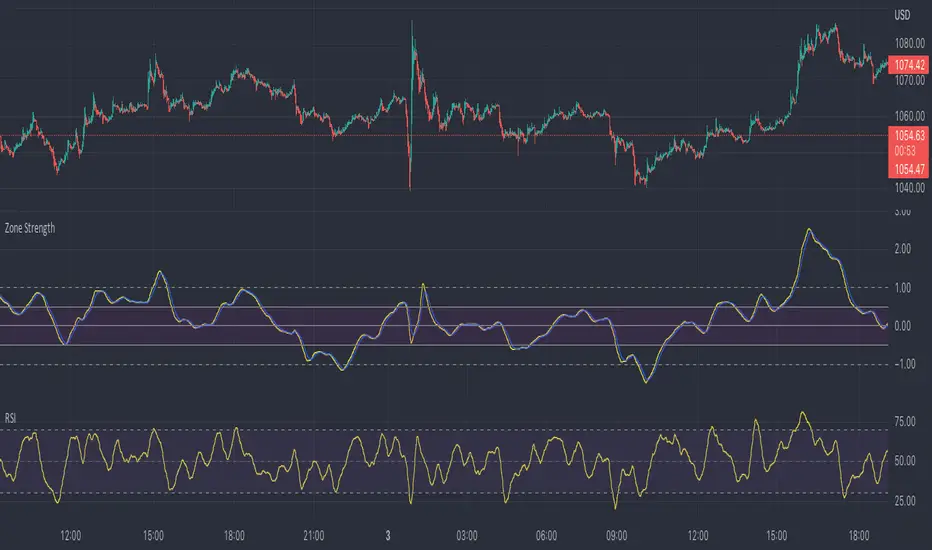
Zone Strength [wbburgin]The Zone Strength indicator is a multifaceted indicator combining volatility-based, momentum-based, and support-based metrics to indicate where a trend reversal is likely.
I recommend using it with the RSI at normal settings to confirm entrances and exits.
The indicator first uses a candle’s wick in relation to its body, depending on whether it closes green or red, to determine ranges of volatility.
The maxima of these volatility statistics are registered across a specific period (the “amplitude”) to determine regions of current support.
The “wavelength” of this statistic is taken to smooth out the Zone Strength’s final statistic.
Finally, the ratio of the difference between the support and the resistance levels is taken in relation to the candle to determine how close the candle is to the “Buy Zone” (<-0.5) or the “Sell Zone” (>0.5).
wbburgin
Daily Short Volume RatioThe short volume ratio is the number of shares sold short divided by the average daily volume and is used to indicate sentiment. In its most basic form, short volume ratio above 0.5 indicates more folks are shorting the stock while a short volume ratio below 0.5 indicates more folks are buying the stock. Short volume and total volume data is collected daily from FINRA for the NYSE and the NASDAQ exchange and represents lit markets. Daily short and total volume is calculated after the exchanges close so will lag by a day on the chart.
This indicator displays the short volume ratio for the last 1, 2, 3, 4, and 5 days and includes a smoothing function (def: off) to better visualize trends.
The indicator also includes the ability to view the short volume ratio for the last day for a reference ticker (def: SPY) to compare with total market sentiment.
Thanks to those before me for providing ideas and code.

Infiten's Price Percentage Oscillator Channel (PPOC Indicator)What is the script used for?
Infiten's Price Percentage Oscillator (PPOC Indicator) can be used as a contrarian indicator for volatile stocks and futures to indicate reversals, areas of support and resistance. For longer term trading, if the Short SMA or prices go above the High PPO Threshold line, it is a sign that the asset is overbought, whereas prices or the Short SMA going below the Low PPO Threshold line indicates that the asset is oversold.
What lines can be plotted?
Low PPO Thresh - Calculated as -PPO Threshold * Short MA + Long MA : Gives the price below which the PPO hits your lower threshold
High PPO Thresh - Calculated as PPO Threshold * Short MA + Long MA : Gives the price above which the PPO hits your upper threshold
MA PPO : Plots candles with the Low PPO Thresh as the low, High PPO Thresh as the high, Short MA as the open, and Long MA as the close.
Short SMA : plots the short simple moving average
Long SMA : plots the long simple moving average
Customizable Values :
Short MA Length : the number of bars back used to calculate the short moving average for a PPO
Long MA Length : the number of bars back used to calculate the long moving average for a PPO
PPO Threshold : the percent difference from the moving average expressed as a decimal (0.5 = 50%)
Recommendations:
Longer timeframes like 300 days are best with larger PPO Thresholds, I recommend using a PPO Threshold of 0.5 or higher. For shorter timeframes like 14 days I recommend setting smaller PPO Thresholds, like 0.3 or lower. I find that these values typically capture the most extremes in price action.
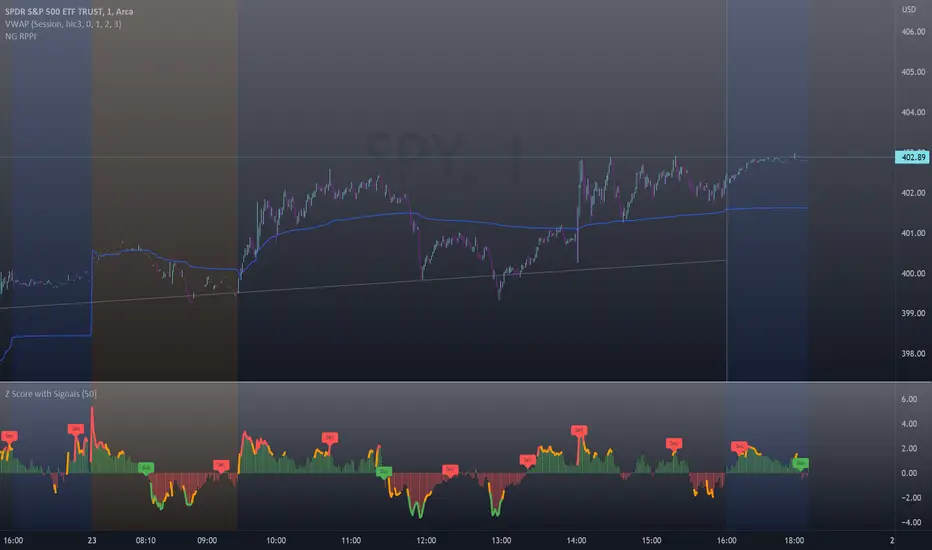
Z-Score with Buy & Sell SignalsThis is my open-source indicator of z-score with buy and sell indicators.
I see there are other z-score indicators, I just am particular about how I like my z-scores calculated and so decided to make my own and add buy and sell signals to help guide me. And I figured I could share it openly here!
What is a Z-Score
A z-score is a statistical measures of the distance, in standard deviations, a value is from its given mean. It is expressed as a standard deviation (or SD). The further a value (in this case, a stock) is from their mean, the more likely a regression to the mean is possible (i.e. a return to the average). So if a stock is trading at 3 standard deviations away from its mean, then we can anticipate it wanting to regress back towards 1 to 0 standard deviations from its mean (i.e. sell off back to a value that brings it closer to that SD).
The inverse is true if it is trading below.
Z-Scores and Stocks
Stocks, like everything in nature, like to trade between -1 and +1 SD away from its mean. Anything above this, we can interpret that there is "stress" on the stock. Anything over 2.50 is tremendous stress on the stock and we can anticipate that it will want to revert to its mean in the near future and bring that value down to at least 1, ideally between the -0.5 and 0.5 range.
Please note, I set the standard VERY high for the indicator to issue a buy and sell signal (/=2.50). Lately with the volatility, stocks have been entering these ranges frequently and so there have been plenty of signals, but traditionally in a stable environment you may not get these signals. I set the bar extremely high because I want to avoid false buy and sell signals (you will still get them though, nothing is perfect!). So the value in this indicator is in interpreting the actual z-score itself, so please be sure you understand exactly what the Z-score is (see the description above).
How the indicator works
The indicator works by calculating the average Z-Score between a stocks high and low. This indicator will present the average deviation a stock has from its high and low average. The higher the Z-Score, the more "overbought" the stock is. The lower the z-score, the more "oversold" the stock is. It uses the previous 500 candles worth of data to calculate its SMA and its Standard deviation in order to calculate the z-score.
Anytime a stock trades 2.50 SDs or more above or below its mean, you will be presented with a Buy or Sell signal, as generally, statistically speaking, after something has travelled 2.50 SDs aware from its mean, there is an increased probability of a reversion happening.
You can use this indicator to determine whether the stock is trading within normal parameters or not and to help you in your analysis as to whether or not a stock could be shorted or longed.
I personally like this for swing trading on the 1 hour chart; however, this can be used on any time from 1 minute to 1 hour. It also allows you to track a stocks progress in its reversion to the mean.
Examples of it in Use:
Gold ETF (ARCA: GLD) on 1 minute
Dow Jones ETF (ARCA: DIA) on 1 minute (my favourite Stock!)
SPY ETF (ARCA: SPY) on 1 hour chart
Disclaimer:
This is not meant to be placed as a sole and single strategy. It should be used in COJUNCTION with your other strategies to help you make a determination.
No indicator is infallible and should never be relied on 100%!
Please let me know your questions/comments/experiences/recommendations below!
Thanks everyone!
HURST Channel StrategyBased on the work TJS / Trading Zoom / Svoboda
Strategy based on Hurst channel with loss averaging when an open position is below 0.5 channel range.
How it works:
1. opens the long position when the close price crosses over the lower band (from bottom to top)
2. opens additional position (double in size) when average position price is lower than average channel value (0.5)
3. closes the position when the close price crosses over the higher band (from top to bottom)
Works the best on :
- volatile and continuous instruments (futures)
- on timeframes above 15 minutes
- uptrends or consolidations
- downtrends require more capital to open double positions

Trend Line RegressionThis is a fast trend line regressor based on least squares regression.
(1) Supports setting regression from the Nth candle
(2) Supports the minimum and maximum regression candle interval length
(3) Supports finding the optimal regression region based on the length step among the minimum and maximum regression region lengths
(4) Supports displaying the optimal regression level
(5) The size of the regression region is 0.5 times the standard deviation by default
(6) You can filter the trend line by setting minimum trend line regression level
(6) Please properly set the parameters to avoid calculation timeout
Enjoy!
这是一个基于最小二乘法回归的快速趋势线回归
(1) 支持从第N根蜡烛开始设置回归
(2) 支持最小和最大的回归蜡烛区间长度
(3) 支持在最小和最大回归区间长度的基础上寻找最佳回归区域
(4) 支持显示最佳回归水平
(5) 回归区域的大小默认为标准差的0.5倍
(6) 可以通过设置最小趋势线回归等级来过滤趋势线
(6) 请正确设置参数以避免计算超时
使用愉快!

Leading Indicator [TH]The leading indicator is helpful to identify early entries and exits (especially near support and resistance).
Green = trend up
Red = trend down
How it works:
The leading indicator calculates the difference between price and an exponential moving average.
Adding the difference creates a negative lag relative to the original function.
Negative lag is what makes this a leading indicator.
The amount of lead is exactly equal to the amount of lag of the moving average.
The leading indicator has lagging signals at turning points.
The leading indicator will always have noise gain, which gets eliminated by applying a moving average.
Modifying the alpha values will modify the amount of noise and change the sensitivity of trend change.
Example 1: Changing alpha1 from 0.25 to 0.15 lowers noise, more clearly identifies trend, and adds delay to this indicator.
Example 2: Changing alpha1 from 0.25 to 0.35 increases noise, less clearly identifies trend, BUT more quickly indicates a trend change.
Calculations:
Where:
alpha1 = 0.25
alpha2 = 0.33
Leading = 2 * (arithmetical mean of current High and Low price) + (alpha1 - 2) * (arithmetical mean of previous High and Low price) + (1 - alpha1) * (previous 'Leading' value)
Total Leading = alpha2 * leading + (1 - alpha2) * (previous 'Total Leading' value)
EMA = 0.5 * (arithmetical mean of previous High and Low price) + 0.5 * (previous 'EMA' value)
Uptrend when 'Total Leading' value is greator than the EMA
Downtrend when 'Total Leading' value is lesser than the EMA
Cybernetic Analysis for Stocks and Futures, by John Ehlers (page 231-235)

WhaleCrew BacktesterBacktesting indicators is easy , just add the following line of code to your script:
plot(longEntry ? 1 : shortEntry ? -1 : longTP ? 0.5 : shortTP ? -0.5 : 0, color=na, editable=false, title='Backtest')
These numbers are defined as constants in the backtester source-code.
After adding this indicator to your chart:
1. Open Settings
2. Select supported indicator to backtest
3. Select if you want to enter Longs and/or Shorts
4. Open the 'Strategy Tester' at the bottom to check the performance
Remember:
past performance is not indicative of future results
repainting indicators will create wrong/unrealistic results

Bat Action Magnet Move BAMM Theory Educational (Source Code)This indicator was intended as educational purpose only for BAMM, which also known as Bat Action Magnet Move.
Indikator ini bertujuan sebagai pendidikan sahaja untuk BAMM, juga dikenali sebagai Bat Action Magnet Move.
BAMM is usually used for Harmonic Patterns such as XAB=CD (Bat Pattern) and AB=CD (0.5 AB=CD Pattern) - Chapter 5.
BAMM also can be used for other Harmonic Pattern with the help of RSI Divergence, hence become RSI BAMM - Chapter 6.
BAMM kebiasaanya digunakan untuk Harmonic Pattern seperti XAB=CD (Bat Pattern) dan AB=CD (0.5 AB=CD Pattern) - Chapter 5.
BAMM juga boleh digunakan untuk Harmonic Pattern lain dengan bantuan RSI Divergence, menjadi RSI BAMM - Chapter 6.
FAQ
1. Credits / Kredit
Scott M Carney,
Scott M Carney, Harmonic Trading: Volume Two (Chapter 5 & Chapter 6)
Bullish XAB=CD BAMM Breakout - Page 144
Bearish XAB=CD BAMM Breakdown - Page 148
Bullish AB=CD BAMM Breakout - Page 153
Bearish AB=CD BAMM Breakdown - Page 156
2. Code Usage / Penggunaan Kod
Free to use for personal usage but credits are most welcomed especially for credits to Scott M Carney.
Bebas untuk kegunaan peribadi tetapi kredit adalah amat dialu-alukan terutamanya kredit kepada Scott M Carney.
2.0 AB=CD Pattern
XAB=CD Bat Pattern