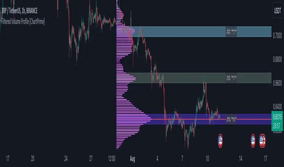
Filtered Volume Profile [ChartPrime]The "Filtered Volume Profile" is a powerful tool that offers insights into market activity. It's a technical analysis tool used to understand the behavior of financial markets. It uses a fixed range volume profile to provide a histogram representing how much volume occurred at distinct price levels.
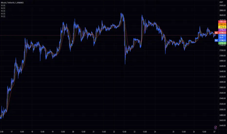
Profile in action with various significant levels displayed
How to Use
The script is designed to analyze cumulative trading volumes in different price bins over a certain period, also known as `'lookback'`. This lookback period can be defined by the user and it represents the number of bars to look back for calculating levels of support and resistance.
The `'Smoothing'` input determines the degree to which the output is smoothed. Higher values lead to smoother results but may impede the responsiveness of the indicator to rapid changes in volatility.
The `'Peak Sensitivity'` input is used to adjust the sensitivity of the script's peak detection algorithm. Setting this to a lower value makes the algorithm more sensitive to local changes in trading volume and may result in "noisier" outputs.
The `'Peak Threshold'` input specifies the number of bins that the peak detection mechanism should account for. Larger numbers imply that more volume bins are taken into account, and the resultant peaks are based on wider intervals.
The `'Mean Score Length'` input is used for scaling the mean score range. This is particularly important in defining the length of lookback bars that will be used to calculate the average close price.
Sinc Filter
The application of the sinc-filter to the Filtered Volume Profile reduces the risk of viewing artefacts that may misrepresent the underlying market behavior. Sinc filtering is a high-quality and sharp filter that doesn't manifest any ringing effects, making it an optimal choice for such volume profiling.
Histogram
On the histogram, the volume profile is colored based on the balance of bullish to bearish volume. If a particular bar is more intense in color, it represents a larger than usual volume during a single price bar. This is a clear signal of a strong buying or selling pressure at a particular price level.
Threshold for Peaks
The `peak_thresh` input determines the number of bins the algorithm takes in account for the peak detection feature. The 'peak' represents the level where a significant amount of volume trading has occurred, and usually is of interest as an indicative of support or resistance level.
By increasing the `peak_thresh`, you're raising the bar for what the algorithm perceives as a peak. This could result in fewer, but more significant peaks being identified.
History of Volume Profiles and Evolution into Sinc Filtering
Volume profiling has a rich history in market analysis, dating back to the 1950s when Richard D. Wyckoff, a legendary trader, introduced the concept of volume studies. He understood the critical significance of volume and its relationship with market price movement. The core of Wyckoff's technical analysis suite was the relationship between prices and volume, often termed as "Effort vs Results".
Moving forward, in the early 1800s, the esteemed mathematician J. R. Carson made key improvements to the sinc function, which formed the basis for sinc filtering application in time series data. Following these contributions, trading studies continued to create and integrate more advanced statistical measures into market analysis.
This culminated in the 1980s with J. Peter Steidlmayer’s introduction of Market Profile. He suggested that markets were a function of continuous two-way auction processes thus introducing the concept of viewing markets in price/time continuum and price distribution forms. Steidlmayer's Market Profile was the first wide-scale operation of organized volume and price data.
However, despite the introduction of such features, challenges in the analysis persisted, especially due to noise that could misinform trading decisions. This gap has given rise to the need for smoothing functions to help eliminate the noise and better interpret the data. Among such techniques, the sinc filter has become widely recognized within the trading community.
The sinc filter, because of its properties of constructing a smooth passing through all data points precisely and its ability to eliminate high-frequency noise, has been considered a natural transition in the evolution of volume profile strategies. The superior ability of the sinc filter to reduce noise and shield against over-fitting makes it an ideal choice for smoothing purposes in trading scripts, particularly where volume profiling forms the crux of the market analysis strategy, such as in Filtered Volume Profile.
Moving ahead, the use of volume-based studies seems likely to remain a core part of technical analysis. As long as markets operate based on supply and demand principles, understanding volume will remain key to discerning the intent behind price movements. And with the incorporation of advanced methods like sinc filtering, the accuracy and insight provided by these methodologies will only improve.
Mean Score
The mean score in the Filtered Volume Profile script plays an important role in probabilistic inferences regarding future price direction. This score essentially characterizes the statistical likelihood of price trends based on historical data.
The mean score is calculated over a configurable `'Mean Score Length'`. This variable sets the window or the timeframe for calculation of the mean score of the closing prices.
Statistically, this score takes advantage of the concept of z-scores and probabilities associated with the t-distribution (a type of probability distribution that is symmetric and bell-shaped, just like the standard normal distribution, but has heavier tails).
The z-score represents how many standard deviations an element is from the mean. In this case, the "element" is the price level (Point of Control).
The mean score section of the script calculates standard errors for the root mean squared error (RMSE) and addresses the uncertainty in the prediction of the future value of a random variable.
The RMSE of a model prediction concerning observed values is used to measure the differences between values predicted by a model and the values observed.
The lower the RMSE, the better the model is able to predict. A zero RMSE means a perfect fit to the data. In essence, it's a measure of how concentrated the data is around the line of best fit.
Through the mean score, the script effectively predicts the likelihood of the future close price being above or below our identified price level.
Summary
Filtered Volume Profile is a comprehensive trading view indicator which utilizes volume profiling, peak detection, mean score computations, and sinc-filter smoothing, altogether providing the finer details of market behavior.
It offers a customizable look back period, smoothing options, and peak sensitivity setting along with a uniquely set peak threshold. The application of the Sinc Filter ensures a high level of accuracy and noise reduction in volume profiling, making this script a reliable tool for gaining market insights.
Furthermore, the use of mean score calculations provides probabilistic insights into price movements, thus providing traders with a statistically sound foundation for their trading decisions. As trading markets advance, the use of such methodologies plays a pivotal role in formulating effective trading strategies and the Filtered Volume Profile is a successful embodiment of such advancements in the field of market analysis.
Chỉ báo Pine Script®