Straight Trend V1Hello everyone,
We are proud to present you our "Straight Trend" Strategy.
Strategy is use a specified timeline's opening price as reference and draw a line between the current price and trend line.
Trend line is smoothed with last X times of highest and lowest values ( Donchian Methodology) in order to create less noise and fake alerts , therefore creates a channel of current prices time based opening price.
The timeline can be adjusted according to your specifications in the settings.
------
Why opening price ?
We are traders ,no matter what we do ,we always make a benchmark at the end of a day , week or at the end of a specified time line.
Example :
X commodity's price increased %15 in last days or Y commodity's price dropped %30 in last 2 weeks etc. etc.
Thats why the opening price have a hidden and much more important role in our trading sessions.
------
After the channel is created we remove the unnecessary lines from our output by filtering the direction with closing price.
IF the closing price is higher than Chanel reference price and direction goes upward the script gives you a BUY signal.
The same methodology is applied for SELL operations.
When to Take Profit?
We put a setting for profit percentage in scripts setting you can adjust the ratio as your choices.
When to Stop Loss or change direction of the trade?
The Straight Trends previously mentioned channel's inverse line was set as STOP LOSS and direction changer in the strategy with "STR-X" Marker.
Note : Strategy is much more effective with heikin-ashi bars due methodology of heikin ashi and with this bars it creates less signals with more accuracy, use at your own discretion.
Please don't hesitate to write us if you need support or assistance, we also appreciate your feedbacks.
Please be advised that this strategy is published with Educational Purposes and it is not a investment advice.
Thank you in advance.
Tìm kiếm tập lệnh với "bands"
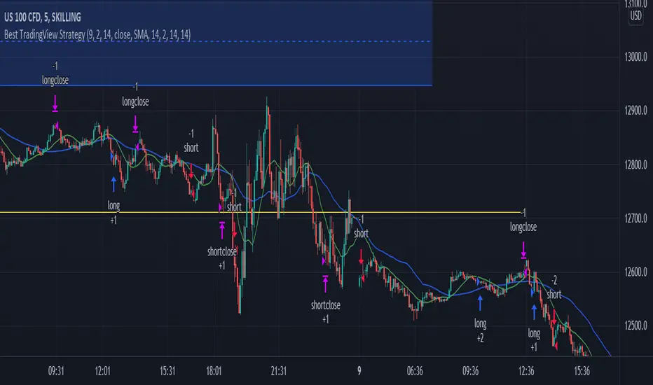
Best TradingView Strategy - For NASDAQ and DOW30 and other IndexThe script is totally based on momentum , volume and price. We have used :
1: Bollinger Band Squeezes to know when a breakout might happen.
2: Used Moving Averages(SMA and EMA) to know the direction.
3: The success Rate of this strategy is above 75% and if little price action is added it can easily surpass 90% success mark.
4: Do not worry about drawdowns , we have implemented trailing SL ,so you might see a little extra drawdown but in reality its pretty less.
5: I myself have tested this strategy for 41 days with a 250$ account and right now I have 2700$.
EHMA Range StrategyThis script is a modified version of @borserman's script for the Exponential Hull Moving Average
All credit for the EHMA goes to him :)
In addition to the EHMA, this script works with a range around the EHMA (which can be modified), in an attempt to be robust against fake signals. Many times a bar will close below a moving average, only to reverse again the next bar, which eats away at your profits. Especially on shorter timeframes, but also on choppy longer timeframes this can make a strategy unattractive to use.
With the range around the EHMA, the strategy only enters a long/exit-short position if a bar crosses above the upper range. Vice versa, it only enters a short/exit-long position if a bar crosses below the lower range. This avoids positions if bars behave choppy within the EHMA range & only enters a position if the market is confident in it's direction. Having said that, fakeouts are still possible, but a lot less frequent. Having backtested this strategy vs the regular EHMA strategy (and having experimented with various settings), this version seems to be a lot more robust & profitable!
Disclaimer
Please remember that past performance may not be indicative of future results.
Due to various factors, including changing market conditions, the strategy may no longer perform as good as in historical backtesting.
This post and the script don’t provide any financial advice.

RSI_Boll-TP/SLThis strategy is originally "Bollinger + RSI , Double Strategy (by ChartArt)"
I added just TP/SL exit point, position direction selection(long, short or both) and time window into that strategy.

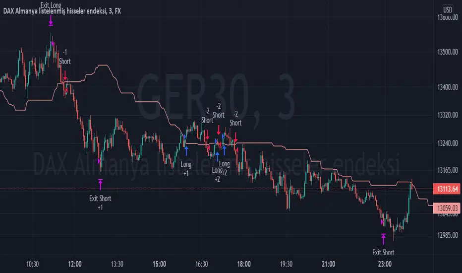
TPS - FX TradeI based my strategy on the Lagging Span 2 line in the Ichimoku Cloud. I actually designed the strategy for the DAX Germany index 3 Minutes period, but you can use it on any instrument you want. I would like to point out some points that you should pay attention to when optimizing the strategy for the instrument you want to use.
Position Take Profit and Stop Loss levels are tick calculations. These values will differ for each instrument. If you are trading in Forex, the values you will write here should be starting from the numbers after the comma in the instrument value. For example, if you want to take profit at "200" points in DAX, you must write "20000" in the Long or Short Take Profit Score field, this applies to the Stop Loss Points, but if you want to take profit or stop loss at 200 points in UKOIL, you must write "200" in the entry part.
Kernel Regression Envelope with SMI OscillatorThis script combines the predictive capabilities of the **Nadaraya-Watson estimator**, implemented by the esteemed jdehorty (credit to him for his excellent work on the `KernelFunctions` library and the original Nadaraya-Watson Envelope indicator), with the confirmation strength of the **Stochastic Momentum Index (SMI)** to create a dynamic trend reversal strategy. The core idea is to identify potential overbought and oversold conditions using the Nadaraya-Watson Envelope and then confirm these signals with the SMI before entering a trade.
**Understanding the Nadaraya-Watson Envelope:**
The Nadaraya-Watson estimator is a non-parametric regression technique that essentially calculates a weighted average of past price data to estimate the current underlying trend. Unlike simple moving averages that give equal weight to all past data within a defined period, the Nadaraya-Watson estimator uses a **kernel function** (in this case, the Rational Quadratic Kernel) to assign weights. The key parameters influencing this estimation are:
* **Lookback Window (h):** This determines how many historical bars are considered for the estimation. A larger window results in a smoother estimation, while a smaller window makes it more reactive to recent price changes.
* **Relative Weighting (alpha):** This parameter controls the influence of different time frames in the estimation. Lower values emphasize longer-term price action, while higher values make the estimator more sensitive to shorter-term movements.
* **Start Regression at Bar (x\_0):** This allows you to exclude the potentially volatile initial bars of a chart from the calculation, leading to a more stable estimation.
The script calculates the Nadaraya-Watson estimation for the closing price (`yhat_close`), as well as the highs (`yhat_high`) and lows (`yhat_low`). The `yhat_close` is then used as the central trend line.
**Dynamic Envelope Bands with ATR:**
To identify potential entry and exit points around the Nadaraya-Watson estimation, the script uses **Average True Range (ATR)** to create dynamic envelope bands. ATR measures the volatility of the price. By multiplying the ATR by different factors (`nearFactor` and `farFactor`), we create multiple bands:
* **Near Bands:** These are closer to the Nadaraya-Watson estimation and are intended to identify potential immediate overbought or oversold zones.
* **Far Bands:** These are further away and can act as potential take-profit or stop-loss levels, representing more extreme price extensions.
The script calculates both near and far upper and lower bands, as well as an average between the near and far bands. This provides a nuanced view of potential support and resistance levels around the estimated trend.
**Confirming Reversals with the Stochastic Momentum Index (SMI):**
While the Nadaraya-Watson Envelope identifies potential overextended conditions, the **Stochastic Momentum Index (SMI)** is used to confirm a potential trend reversal. The SMI, unlike a traditional stochastic oscillator, oscillates around a zero line. It measures the location of the current closing price relative to the median of the high/low range over a specified period.
The script calculates the SMI on a **higher timeframe** (defined by the "Timeframe" input) to gain a broader perspective on the market momentum. This helps to filter out potential whipsaws and false signals that might occur on the current chart's timeframe. The SMI calculation involves:
* **%K Length:** The lookback period for calculating the highest high and lowest low.
* **%D Length:** The period for smoothing the relative range.
* **EMA Length:** The period for smoothing the SMI itself.
The script uses a double EMA for smoothing within the SMI calculation for added smoothness.
**How the Indicators Work Together in the Strategy:**
The strategy enters a long position when:
1. The closing price crosses below the **near lower band** of the Nadaraya-Watson Envelope, suggesting a potential oversold condition.
2. The SMI crosses above its EMA, indicating positive momentum.
3. The SMI value is below -50, further supporting the oversold idea on the higher timeframe.
Conversely, the strategy enters a short position when:
1. The closing price crosses above the **near upper band** of the Nadaraya-Watson Envelope, suggesting a potential overbought condition.
2. The SMI crosses below its EMA, indicating negative momentum.
3. The SMI value is above 50, further supporting the overbought idea on the higher timeframe.
Trades are closed when the price crosses the **far band** in the opposite direction of the trade. A stop-loss is also implemented based on a fixed value.
**In essence:** The Nadaraya-Watson Envelope identifies areas where the price might be deviating significantly from its estimated trend. The SMI, calculated on a higher timeframe, then acts as a confirmation signal, suggesting that the momentum is shifting in the direction of a potential reversal. The ATR-based bands provide dynamic entry and exit points based on the current volatility.
**How to Use the Script:**
1. **Apply the script to your chart.**
2. **Adjust the "Kernel Settings":**
* **Lookback Window (h):** Experiment with different values to find the smoothness that best suits the asset and timeframe you are trading. Lower values make the envelope more reactive, while higher values make it smoother.
* **Relative Weighting (alpha):** Adjust to control the influence of different timeframes on the Nadaraya-Watson estimation.
* **Start Regression at Bar (x\_0):** Increase this value if you want to exclude the initial, potentially volatile, bars from the calculation.
* **Stoploss:** Set your desired stop-loss value.
3. **Adjust the "SMI" settings:**
* **%K Length, %D Length, EMA Length:** These parameters control the sensitivity and smoothness of the SMI. Experiment to find settings that work well for your trading style.
* **Timeframe:** Select the higher timeframe you want to use for SMI confirmation.
4. **Adjust the "ATR Length" and "Near/Far ATR Factor":** These settings control the width and sensitivity of the envelope bands. Smaller ATR lengths make the bands more reactive to recent volatility.
5. **Customize the "Color Settings"** to your preference.
6. **Observe the plots:**
* The **Nadaraya-Watson Estimation (yhat)** line represents the estimated underlying trend.
* The **near and far upper and lower bands** visualize potential overbought and oversold zones based on the ATR.
* The **fill areas** highlight the regions between the near and far bands.
7. **Look for entry signals:** A long entry is considered when the price touches or crosses below the lower near band and the SMI confirms upward momentum. A short entry is considered when the price touches or crosses above the upper near band and the SMI confirms downward momentum.
8. **Manage your trades:** The script provides exit signals when the price crosses the far band. The fixed stop-loss will also close trades if the price moves against your position.
**Justification for Combining Nadaraya-Watson Envelope and SMI:**
The combination of the Nadaraya-Watson Envelope and the SMI provides a more robust approach to identifying potential trend reversals compared to using either indicator in isolation. The Nadaraya-Watson Envelope excels at identifying potential areas where the price is overextended relative to its recent history. However, relying solely on the envelope can lead to false signals, especially in choppy or volatile markets. By incorporating the SMI as a confirmation tool, we add a momentum filter that helps to validate the potential reversals signaled by the envelope. The higher timeframe SMI further helps to filter out noise and focus on more significant shifts in momentum. The ATR-based bands add a dynamic element to the entry and exit points, adapting to the current market volatility. This mashup aims to leverage the strengths of each indicator to create a more reliable trading strategy.

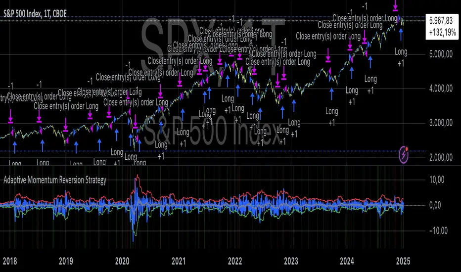
Adaptive Momentum Reversion StrategyThe Adaptive Momentum Reversion Strategy: An Empirical Approach to Market Behavior
The Adaptive Momentum Reversion Strategy seeks to capitalize on market price dynamics by combining concepts from momentum and mean reversion theories. This hybrid approach leverages a Rate of Change (ROC) indicator along with Bollinger Bands to identify overbought and oversold conditions, triggering trades based on the crossing of specific thresholds. The strategy aims to detect momentum shifts and exploit price reversions to their mean.
Theoretical Framework
Momentum and Mean Reversion: Momentum trading assumes that assets with a recent history of strong performance will continue in that direction, while mean reversion suggests that assets tend to return to their historical average over time (Fama & French, 1988; Poterba & Summers, 1988). This strategy incorporates elements of both, looking for periods when momentum is either overextended (and likely to revert) or when the asset’s price is temporarily underpriced relative to its historical trend.
Rate of Change (ROC): The ROC is a straightforward momentum indicator that measures the percentage change in price over a specified period (Wilder, 1978). The strategy calculates the ROC over a 2-period window, making it responsive to short-term price changes. By using ROC, the strategy aims to detect price acceleration and deceleration.
Bollinger Bands: Bollinger Bands are used to identify volatility and potential price extremes, often signaling overbought or oversold conditions. The bands consist of a moving average and two standard deviation bounds that adjust dynamically with price volatility (Bollinger, 2002).
The strategy employs two sets of Bollinger Bands: one for short-term volatility (lower band) and another for longer-term trends (upper band), with different lengths and standard deviation multipliers.
Strategy Construction
Indicator Inputs:
ROC Period: The rate of change is computed over a 2-period window, which provides sensitivity to short-term price fluctuations.
Bollinger Bands:
Lower Band: Calculated with a 18-period length and a standard deviation of 1.7.
Upper Band: Calculated with a 21-period length and a standard deviation of 2.1.
Calculations:
ROC Calculation: The ROC is computed by comparing the current close price to the close price from rocPeriod days ago, expressing it as a percentage.
Bollinger Bands: The strategy calculates both upper and lower Bollinger Bands around the ROC, using a simple moving average as the central basis. The lower Bollinger Band is used as a reference for identifying potential long entry points when the ROC crosses above it, while the upper Bollinger Band serves as a reference for exits, when the ROC crosses below it.
Trading Conditions:
Long Entry: A long position is initiated when the ROC crosses above the lower Bollinger Band, signaling a potential shift from a period of low momentum to an increase in price movement.
Exit Condition: A position is closed when the ROC crosses under the upper Bollinger Band, or when the ROC drops below the lower band again, indicating a reversal or weakening of momentum.
Visual Indicators:
ROC Plot: The ROC is plotted as a line to visualize the momentum direction.
Bollinger Bands: The upper and lower bands, along with their basis (simple moving averages), are plotted to delineate the expected range for the ROC.
Background Color: To enhance decision-making, the strategy colors the background when extreme conditions are detected—green for oversold (ROC below the lower band) and red for overbought (ROC above the upper band), indicating potential reversal zones.
Strategy Performance Considerations
The use of Bollinger Bands in this strategy provides an adaptive framework that adjusts to changing market volatility. When volatility increases, the bands widen, allowing for larger price movements, while during quieter periods, the bands contract, reducing trade signals. This adaptiveness is critical in maintaining strategy effectiveness across different market conditions.
The strategy’s pyramiding setting is disabled (pyramiding=0), ensuring that only one position is taken at a time, which is a conservative risk management approach. Additionally, the strategy includes transaction costs and slippage parameters to account for real-world trading conditions.
Empirical Evidence and Relevance
The combination of momentum and mean reversion has been widely studied and shown to provide profitable opportunities under certain market conditions. Studies such as Jegadeesh and Titman (1993) confirm that momentum strategies tend to work well in trending markets, while mean reversion strategies have been effective during periods of high volatility or after sharp price movements (De Bondt & Thaler, 1985). By integrating both strategies into one system, the Adaptive Momentum Reversion Strategy may be able to capitalize on both trending and reverting market behavior.
Furthermore, research by Chan (1996) on momentum-based trading systems demonstrates that adaptive strategies, which adjust to changes in market volatility, often outperform static strategies, providing a compelling rationale for the use of Bollinger Bands in this context.
Conclusion
The Adaptive Momentum Reversion Strategy provides a robust framework for trading based on the dual concepts of momentum and mean reversion. By using ROC in combination with Bollinger Bands, the strategy is capable of identifying overbought and oversold conditions while adapting to changing market conditions. The use of adaptive indicators ensures that the strategy remains flexible and can perform across different market environments, potentially offering a competitive edge for traders who seek to balance risk and reward in their trading approaches.
References
Bollinger, J. (2002). Bollinger on Bollinger Bands. McGraw-Hill Professional.
Chan, L. K. C. (1996). Momentum, Mean Reversion, and the Cross-Section of Stock Returns. Journal of Finance, 51(5), 1681-1713.
De Bondt, W. F., & Thaler, R. H. (1985). Does the Stock Market Overreact? Journal of Finance, 40(3), 793-805.
Fama, E. F., & French, K. R. (1988). Permanent and Temporary Components of Stock Prices. Journal of Political Economy, 96(2), 246-273.
Jegadeesh, N., & Titman, S. (1993). Returns to Buying Winners and Selling Losers: Implications for Stock Market Efficiency. Journal of Finance, 48(1), 65-91.
Poterba, J. M., & Summers, L. H. (1988). Mean Reversion in Stock Prices: Evidence and Implications. Journal of Financial Economics, 22(1), 27-59.
Wilder, J. W. (1978). New Concepts in Technical Trading Systems. Trend Research.
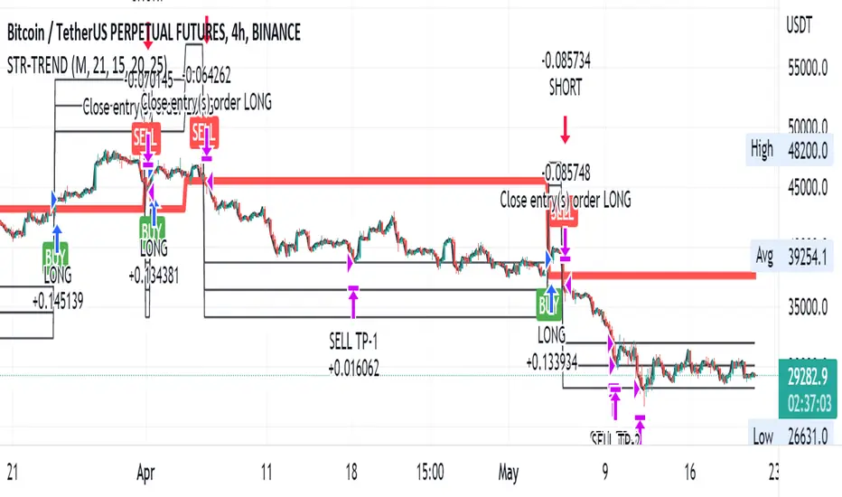
Follow Line Strategy Version 2.5 (React HTF)Follow Line Strategy v2.5 (React HTF) - TradingView Script Usage
This strategy utilizes a "Follow Line" concept based on Bollinger Bands and ATR to identify potential trading opportunities. It includes advanced features like optional working hours filtering, higher timeframe (HTF) trend confirmation, and improved trend-following entry/exit logic. Version 2.5 introduces reactivity to HTF trend changes for more adaptive trading.
Key Features:
Follow Line: The core of the strategy. It dynamically adjusts based on price breakouts beyond Bollinger Bands, using either the low/high or ATR-adjusted levels.
Bollinger Bands: Uses a standard Bollinger Bands setup to identify overbought/oversold conditions.
ATR Filter: Optionally uses the Average True Range (ATR) to adjust the Follow Line offset, providing a more dynamic and volatility-adjusted entry point.
Optional Trading Session Filter: Allows you to restrict trading to specific hours of the day.
Higher Timeframe (HTF) Confirmation: A significant feature that allows you to confirm trade signals with the trend on a higher timeframe. This can help to filter out false signals and improve the overall win rate.
HTF Selection Method: Choose between Auto and Manual HTF selection:
Auto: The script automatically determines the appropriate HTF based on the current chart timeframe (e.g., 1min -> 15min, 5min -> 4h, 1h -> 1D, Daily -> Monthly).
Manual: Allows you to select a specific HTF using the Manual Higher Timeframe input.
Trend-Following Entries/Exits: The strategy aims to enter trades in the direction of the established trend, using the Follow Line to define the trend.
Reactive HTF Trend Changes: v2.5 exits positions not only based on the trade timeframe (TTF) trend changing, but also when the higher timeframe trend reverses against the position. This makes the strategy more responsive to larger market movements.
Alerts: Provides buy and sell alerts for convenient trading signal notifications.
Visualizations: Plots the Follow Line for both the trade timeframe and the higher timeframe (optional), making it easy to understand the strategy's logic.
How to Use:
Add to Chart: Add the "Follow Line Strategy Version 2.5 (React HTF)" script to your TradingView chart.
Configure Settings: Customize the strategy's settings to match your trading style and preferences. Here's a breakdown of the key settings:
Indicator Settings:
ATR Period: The period used to calculate the ATR. A smaller period is more sensitive to recent price changes.
Bollinger Bands Period: The period used for the Bollinger Bands calculation. A longer period results in smoother bands.
Bollinger Bands Deviation: The number of standard deviations from the moving average that the Bollinger Bands are plotted. Higher deviations create wider bands.
Use ATR for Follow Line Offset?: Enable to use ATR to calculate the Follow Line offset. Disable to use the simple high/low.
Show Trade Signals on Chart?: Enable to show BUY/SELL labels on the chart.
Time Filter:
Use Trading Session Filter?: Enable to restrict trading to specific hours of the day.
Trading Session: The trading session to use (e.g., 0930-1600 for regular US stock market hours). Use 0000-2400 for all hours.
Higher Timeframe Confirmation:
Enable HTF Confirmation?: Enable to use the HTF trend to filter trade signals. If enabled, only trades in the direction of the HTF trend will be taken.
HTF Selection Method: Choose between "Auto" and "Manual" HTF selection.
Manual Higher Timeframe: If "Manual" is selected, choose the specific HTF (e.g., 240 for 4 hours, D for daily).
Show HTF Follow Line?: Enable to plot the HTF Follow Line on the chart.
Understanding the Signals:
Buy Signal: The price breaks above the upper Bollinger Band, and the HTF (if enabled) confirms the uptrend.
Sell Signal: The price breaks below the lower Bollinger Band, and the HTF (if enabled) confirms the downtrend.
Exit Long: The trade timeframe trend changes to downtrend or the higher timeframe trend changes to downtrend.
Exit Short: The trade timeframe trend changes to uptrend or the higher timeframe trend changes to uptrend.
Alerts:
The script includes alert conditions for buy and sell signals. To set up alerts, click the "Alerts" button in TradingView and select the desired alert condition from the script. The alert message provides the ticker and interval.
Backtesting and Optimization:
Use TradingView's Strategy Tester to backtest the strategy on different assets and timeframes.
Experiment with different settings to optimize the strategy for your specific trading style and risk tolerance. Pay close attention to the ATR Period, Bollinger Bands settings, and the HTF confirmation options.
Tips and Considerations:
HTF Confirmation: The HTF confirmation can significantly improve the strategy's performance by filtering out false signals. However, it can also reduce the number of trades.
Risk Management: Always use proper risk management techniques, such as stop-loss orders and position sizing, when trading any strategy.
Market Conditions: The strategy may perform differently in different market conditions. It's important to backtest and optimize the strategy for the specific markets you are trading.
Customization: Feel free to modify the script to suit your specific needs. For example, you could add additional filters or entry/exit conditions.
Pyramiding: The pyramiding = 0 setting prevents multiple entries in the same direction, ensuring the strategy doesn't compound losses. You can adjust this value if you prefer to pyramid into winning positions, but be cautious.
Lookahead: The lookahead = barmerge.lookahead_off setting ensures that the HTF data is calculated based on the current bar's closed data, preventing potential future peeking bias.
Trend Determination: The logic for determining the HTF trend and reacting to changes is critical. Carefully review the f_calculateHTFData function and the conditions for exiting positions to ensure you understand how the strategy responds to different market scenarios.
Disclaimer:
This script is for informational and educational purposes only. It is not financial advice, and you should not trade based solely on the signals generated by this script. Always do your own research and consult with a qualified financial advisor before making any trading decisions. The author is not responsible for any losses incurred as a result of using this script.

Multi-Regression StrategyIntroducing the "Multi-Regression Strategy" (MRS) , an advanced technical analysis tool designed to provide flexible and robust market analysis across various financial instruments.
This strategy offers users the ability to select from multiple regression techniques and risk management measures, allowing for customized analysis tailored to specific market conditions and trading styles.
Core Components:
Regression Techniques:
Users can choose one of three regression methods:
1 - Linear Regression: Provides a straightforward trend line, suitable for steady markets.
2 - Ridge Regression: Offers a more stable trend estimation in volatile markets by introducing a regularization parameter (lambda).
3 - LOESS (Locally Estimated Scatterplot Smoothing): Adapts to non-linear trends, useful for complex market behaviors.
Each regression method calculates a trend line that serves as the basis for trading decisions.
Risk Management Measures:
The strategy includes nine different volatility and trend strength measures. Users select one to define the trading bands:
1 - ATR (Average True Range)
2 - Standard Deviation
3 - Bollinger Bands Width
4 - Keltner Channel Width
5 - Chaikin Volatility
6 - Historical Volatility
7 - Ulcer Index
8 - ATRP (ATR Percentage)
9 - KAMA Efficiency Ratio
The chosen measure determines the width of the bands around the regression line, adapting to market volatility.
How It Works:
Regression Calculation:
The selected regression method (Linear, Ridge, or LOESS) calculates the main trend line.
For Ridge Regression, users can adjust the lambda parameter for regularization.
LOESS allows customization of the point span, adaptiveness, and exponent for local weighting.
Risk Band Calculation:
The chosen risk measure is calculated and normalized.
A user-defined risk multiplier is applied to adjust the sensitivity.
Upper and lower bounds are created around the regression line based on this risk measure.
Trading Signals:
Long entries are triggered when the price crosses above the regression line.
Short entries occur when the price crosses below the regression line.
Optional stop-loss and take-profit mechanisms use the calculated risk bands.
Customization and Flexibility:
Users can switch between regression methods to adapt to different market trends (linear, regularized, or non-linear).
The choice of risk measure allows adaptation to various market volatility conditions.
Adjustable parameters (e.g., regression length, risk multiplier) enable fine-tuning of the strategy.
Unique Aspects:
Comprehensive Regression Options:
Unlike many indicators that rely on a single regression method, MRS offers three distinct techniques, each suitable for different market conditions.
Diverse Risk Measures: The strategy incorporates a wide range of volatility and trend strength measures, going beyond traditional indicators to provide a more nuanced view of market dynamics.
Unified Framework:
By combining advanced regression techniques with various risk measures, MRS offers a cohesive approach to trend identification and risk management.
Adaptability:
The strategy can be easily adjusted to suit different trading styles, timeframes, and market conditions through its various input options.
How to Use:
Select a regression method based on your analysis of the current market trend (linear, need for regularization, or non-linear).
Choose a risk measure that aligns with your trading style and the market's current volatility characteristics.
Adjust the length parameter to match your preferred timeframe for analysis.
Fine-tune the risk multiplier to set the desired sensitivity of the trading bands.
Optionally enable stop-loss and take-profit mechanisms using the calculated risk bands.
Monitor the regression line for potential trend changes and the risk bands for entry/exit signals.
By offering this level of customization within a unified framework, the Multi-Regression Strategy provides traders with a powerful tool for market analysis and trading decision support. It combines the robustness of regression analysis with the adaptability of various risk measures, allowing for a more comprehensive and flexible approach to technical trading.

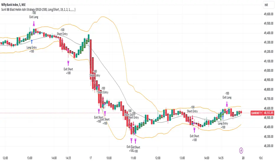
Sunil BB Blast Heikin Ashi StrategySunil BB Blast Heikin Ashi Strategy
The Sunil BB Blast Heikin Ashi Strategy is a trend-following trading strategy that combines Bollinger Bands with Heikin-Ashi candles for precise market entries and exits. It aims to capitalize on price volatility while ensuring controlled risk through dynamic stop-loss and take-profit levels based on a user-defined Risk-to-Reward Ratio (RRR).
Key Features:
Trading Window:
The strategy operates within a user-defined time window (e.g., from 09:20 to 15:00) to align with market hours or other preferred trading sessions.
Trade Direction:
Users can select between Long Only, Short Only, or Long/Short trade directions, allowing flexibility depending on market conditions.
Bollinger Bands:
Bollinger Bands are used to identify potential breakout or breakdown zones. The strategy enters trades when price breaks through the upper or lower Bollinger Band, indicating a possible trend continuation.
Heikin-Ashi Candles:
Heikin-Ashi candles help smooth price action and filter out market noise. The strategy uses these candles to confirm trend direction and improve entry accuracy.
Risk Management (Risk-to-Reward Ratio):
The strategy automatically adjusts the take-profit (TP) level and stop-loss (SL) based on the selected Risk-to-Reward Ratio (RRR). This ensures that trades are risk-managed effectively.
Automated Alerts and Webhooks:
The strategy includes automated alerts for trade entries and exits. Users can set up JSON webhooks for external execution or trading automation.
Active Position Tracking:
The strategy tracks whether there is an active position (long or short) and only exits when price hits the pre-defined SL or TP levels.
Exit Conditions:
The strategy exits positions when either the take-profit (TP) or stop-loss (SL) levels are hit, ensuring risk management is adhered to.
Default Settings:
Trading Window:
09:20-15:00
This setting confines the strategy to the specified hours, ensuring trading only occurs during active market hours.
Strategy Direction:
Default: Long/Short
This allows for both long and short trades depending on market conditions. You can select "Long Only" or "Short Only" if you prefer to trade in one direction.
Bollinger Band Length (bbLength):
Default: 19
Length of the moving average used to calculate the Bollinger Bands.
Bollinger Band Multiplier (bbMultiplier):
Default: 2.0
Multiplier used to calculate the upper and lower bands. A higher multiplier increases the width of the bands, leading to fewer but more significant trades.
Take Profit Multiplier (tpMultiplier):
Default: 2.0
Multiplier used to determine the take-profit level based on the calculated stop-loss. This ensures that the profit target aligns with the selected Risk-to-Reward Ratio.
Risk-to-Reward Ratio (RRR):
Default: 1.0
The ratio used to calculate the take-profit relative to the stop-loss. A higher RRR means larger profit targets.
Trade Automation (JSON Webhooks):
Allows for integration with external systems for automated execution:
Long Entry JSON: Customizable entry condition for long positions.
Long Exit JSON: Customizable exit condition for long positions.
Short Entry JSON: Customizable entry condition for short positions.
Short Exit JSON: Customizable exit condition for short positions.
Entry Logic:
Long Entry:
The strategy enters a long position when:
The Heikin-Ashi candle shows a bullish trend (green close > open).
The price is above the upper Bollinger Band, signaling a breakout.
The previous candle also closed higher than it opened.
Short Entry:
The strategy enters a short position when:
The Heikin-Ashi candle shows a bearish trend (red close < open).
The price is below the lower Bollinger Band, signaling a breakdown.
The previous candle also closed lower than it opened.
Exit Logic:
Take-Profit (TP):
The take-profit level is calculated as a multiple of the distance between the entry price and the stop-loss level, determined by the selected Risk-to-Reward Ratio (RRR).
Stop-Loss (SL):
The stop-loss is placed at the opposite Bollinger Band level (lower for long positions, upper for short positions).
Exit Trigger:
The strategy exits a trade when either the take-profit or stop-loss level is hit.
Plotting and Visuals:
The Heikin-Ashi candles are displayed on the chart, with green candles for uptrends and red candles for downtrends.
Bollinger Bands (upper, lower, and basis) are plotted for visual reference.
Entry points for long and short trades are marked with green and red labels below and above bars, respectively.
Strategy Alerts:
Alerts are triggered when:
A long entry condition is met.
A short entry condition is met.
A trade exits (either via take-profit or stop-loss).
These alerts can be used to trigger notifications or webhook events for automated trading systems.
Notes:
The strategy is designed for use on intraday charts but can be applied to any timeframe.
It is highly customizable, allowing for tailored risk management and trading windows.
The Sunil BB Blast Heikin Ashi Strategy combines two powerful technical analysis tools (Bollinger Bands and Heikin-Ashi candles) with strong risk management, making it suitable for both beginners and experienced traders.
Feebacks are welcome from the users.
Trend Deviation strategy - BTC [IkkeOmar]Intro:
This is an example if anyone needs a push to get started with making strategies in pine script. This is an example on BTC, obviously it isn't a good strategy, and I wouldn't share my own good strategies because of alpha decay.
This strategy integrates several technical indicators to determine market trends and potential trade setups. These indicators include:
Directional Movement Index (DMI)
Bollinger Bands (BB)
Schaff Trend Cycle (STC)
Moving Average Convergence Divergence (MACD)
Momentum Indicator
Aroon Indicator
Supertrend Indicator
Relative Strength Index (RSI)
Exponential Moving Average (EMA)
Volume Weighted Average Price (VWAP)
It's crucial for you guys to understand the strengths and weaknesses of each indicator and identify synergies between them to improve the strategy's effectiveness.
Indicator Settings:
DMI (Directional Movement Index):
Length: This parameter determines the number of bars used in calculating the DMI. A higher length may provide smoother results but might lag behind the actual price action.
Bollinger Bands:
Length: This parameter specifies the number of bars used to calculate the moving average for the Bollinger Bands. A longer length results in a smoother average but might lag behind the price action.
Multiplier: The multiplier determines the width of the Bollinger Bands. It scales the standard deviation of the price data. A higher multiplier leads to wider bands, indicating increased volatility, while a lower multiplier results in narrower bands, suggesting decreased volatility.
Schaff Trend Cycle (STC):
Length: This parameter defines the length of the STC calculation. A longer length may result in smoother but slower-moving signals.
Fast Length: Specifies the length of the fast moving average component in the STC calculation.
Slow Length: Specifies the length of the slow moving average component in the STC calculation.
MACD (Moving Average Convergence Divergence):
Fast Length: Determines the number of bars used to calculate the fast EMA (Exponential Moving Average) in the MACD.
Slow Length: Specifies the number of bars used to calculate the slow EMA in the MACD.
Signal Length: Defines the number of bars used to calculate the signal line, which is typically an EMA of the MACD line.
Momentum Indicator:
Length: This parameter sets the number of bars over which momentum is calculated. A longer length may provide smoother momentum readings but might lag behind significant price changes.
Aroon Indicator:
Length: Specifies the number of bars over which the Aroon indicator calculates its values. A longer length may result in smoother Aroon readings but might lag behind significant market movements.
Supertrend Indicator:
Trendline Length: Determines the length of the period used in the Supertrend calculation. A longer length results in a smoother trendline but might lag behind recent price changes.
Trendline Factor: Specifies the multiplier used in calculating the trendline. It affects the sensitivity of the indicator to price changes.
RSI (Relative Strength Index):
Length: This parameter sets the number of bars over which RSI calculates its values. A longer length may result in smoother RSI readings but might lag behind significant price changes.
EMA (Exponential Moving Average):
Fast EMA: Specifies the number of bars used to calculate the fast EMA. A shorter period results in a more responsive EMA to recent price changes.
Slow EMA: Determines the number of bars used to calculate the slow EMA. A longer period results in a smoother EMA but might lag behind recent price changes.
VWAP (Volume Weighted Average Price):
Default settings are typically used for VWAP calculations, which consider the volume traded at each price level over a specific period. This indicator provides insights into the average price weighted by trading volume.
backtest range and rules:
You can specify the start date for backtesting purposes.
You can can select the desired trade direction: Long, Short, or Both.
Entry and Exit Conditions:
LONG:
DMI Cross Up: The Directional Movement Index (DMI) indicates a bullish trend when the positive directional movement (+DI) crosses above the negative directional movement (-DI).
Bollinger Bands (BB): The price is below the upper Bollinger Band, indicating a potential reversal from the upper band.
Momentum Indicator: Momentum is positive, suggesting increasing buying pressure.
MACD (Moving Average Convergence Divergence): The MACD line is above the signal line, indicating bullish momentum.
Supertrend Indicator: The Supertrend indicator signals an uptrend.
Schaff Trend Cycle (STC): The STC indicates a bullish trend.
Aroon Indicator: The Aroon indicator signals a bullish trend or crossover.
When all these conditions are met simultaneously, the strategy considers it a favorable opportunity to enter a long trade.
SHORT:
DMI Cross Down: The Directional Movement Index (DMI) indicates a bearish trend when the negative directional movement (-DI) crosses above the positive directional movement (+DI).
Bollinger Bands (BB): The price is above the lower Bollinger Band, suggesting a potential reversal from the lower band.
Momentum Indicator: Momentum is negative, indicating increasing selling pressure.
MACD (Moving Average Convergence Divergence): The MACD line is below the signal line, signaling bearish momentum.
Supertrend Indicator: The Supertrend indicator signals a downtrend.
Schaff Trend Cycle (STC): The STC indicates a bearish trend.
Aroon Indicator: The Aroon indicator signals a bearish trend or crossover.
When all these conditions align, the strategy considers it an opportune moment to enter a short trade.
Disclaimer:
THIS ISN'T AN OPTIMAL STRATEGY AT ALL! It was just an old project from when I started learning pine script!
The backtest doesn't promise the same results in the future, always do both in-sample and out-of-sample testing when backtesting a strategy. And make sure you forward test it as well before implementing it!
Furthermore this strategy uses both trend and mean-reversion systems, that is usually a no-go if you want to build robust trend systems .
Don't hesitate to comment if you have any questions or if you have some good notes for a beginner.

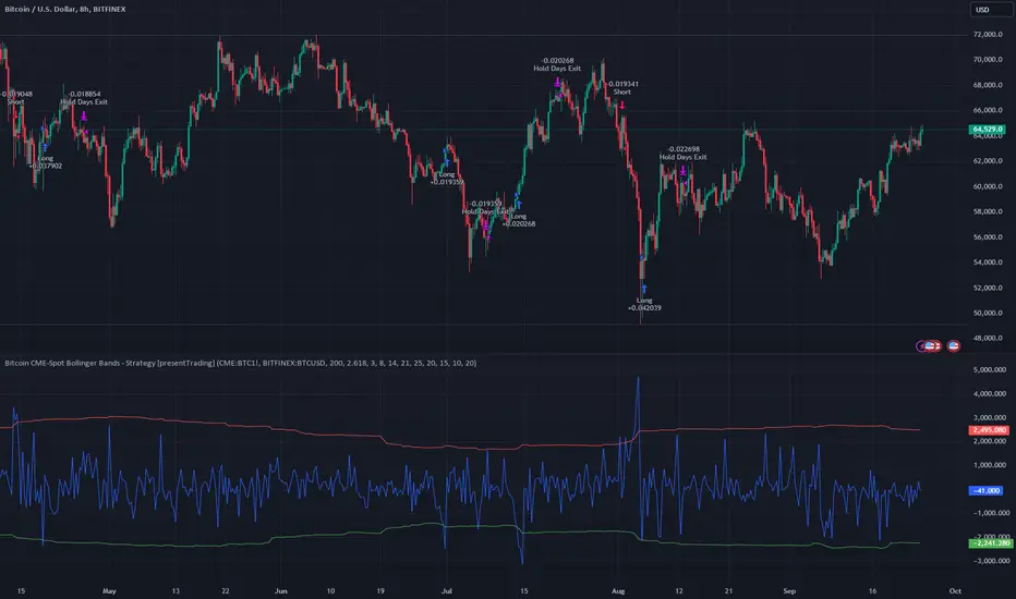
Bitcoin CME-Spot Z-Spread - Strategy [presentTrading]This time is a swing trading strategy! It measures the sentiment of the Bitcoin market through the spread of CME Bitcoin Futures and Bitfinex BTCUSD Spot prices. By applying Bollinger Bands to the spread, the strategy seeks to capture mean-reversion opportunities when prices deviate significantly from their historical norms
█ Introduction and How it is Different
The Bitcoin CME-Spot Bollinger Bands Strategy is designed to capture mean-reversion opportunities by exploiting the spread between CME Bitcoin Futures and Bitfinex BTCUSD Spot prices. The strategy uses Bollinger Bands to detect when the spread between these two correlated assets has deviated significantly from its historical norm, signaling potential overbought or oversold conditions.
What sets this strategy apart is its focus on spread trading between futures and spot markets rather than price-based indicators. By applying Bollinger Bands to the spread rather than individual prices, the strategy identifies price inefficiencies across markets, allowing traders to take advantage of the natural reversion to the mean that often occurs in these correlated assets.
BTCUSD 8hr Performance
█ Strategy, How It Works: Detailed Explanation
The strategy relies on Bollinger Bands to assess the volatility and relative deviation of the spread between CME Bitcoin Futures and Bitfinex BTCUSD Spot prices. Bollinger Bands consist of a moving average and two standard deviation bands, which help measure how much the spread deviates from its historical mean.
🔶 Spread Calculation:
The spread is calculated by subtracting the Bitfinex spot price from the CME Bitcoin futures price:
Spread = CME Price - Bitfinex Price
This spread represents the difference between the futures and spot markets, which may widen or narrow based on supply and demand dynamics in each market. By analyzing the spread, the strategy can detect when prices are too far apart (potentially overbought or oversold), indicating a trading opportunity.
🔶 Bollinger Bands Calculation:
The Bollinger Bands for the spread are calculated using a simple moving average (SMA) and the standard deviation of the spread over a defined period.
1. Moving Average (SMA):
The simple moving average of the spread (mu_S) over a specified period P is calculated as:
mu_S = (1/P) * sum(S_i from i=1 to P)
Where S_i represents the spread at time i, and P is the lookback period (default is 200 bars). The moving average provides a baseline for the normal spread behavior.
2. Standard Deviation:
The standard deviation (sigma_S) of the spread is calculated to measure the volatility of the spread:
sigma_S = sqrt((1/P) * sum((S_i - mu_S)^2 from i=1 to P))
3. Upper and Lower Bollinger Bands:
The upper and lower Bollinger Bands are derived by adding and subtracting a multiple of the standard deviation from the moving average. The number of standard deviations is determined by a user-defined parameter k (default is 2.618).
- Upper Band:
Upper Band = mu_S + (k * sigma_S)
- Lower Band:
Lower Band = mu_S - (k * sigma_S)
These bands provide a dynamic range within which the spread typically fluctuates. When the spread moves outside of these bands, it is considered overbought or oversold, potentially offering trading opportunities.
Local view
🔶 Entry Conditions:
- Long Entry: A long position is triggered when the spread crosses below the lower Bollinger Band, indicating that the spread has become oversold and is likely to revert upward.
Spread < Lower Band
- Short Entry: A short position is triggered when the spread crosses above the upper Bollinger Band, indicating that the spread has become overbought and is likely to revert downward.
Spread > Upper Band
🔶 Risk Management and Profit-Taking:
The strategy incorporates multi-step take profits to lock in gains as the trade moves in favor. The position is gradually reduced at predefined profit levels, reducing risk while allowing part of the trade to continue running if the price keeps moving favorably.
Additionally, the strategy uses a hold period exit mechanism. If the trade does not hit any of the take-profit levels within a certain number of bars, the position is closed automatically to avoid excessive exposure to market risks.
█ Trade Direction
The trade direction is based on deviations of the spread from its historical norm:
- Long Trade: The strategy enters a long position when the spread crosses below the lower Bollinger Band, signaling an oversold condition where the spread is expected to narrow.
- Short Trade: The strategy enters a short position when the spread crosses above the upper Bollinger Band, signaling an overbought condition where the spread is expected to widen.
These entries rely on the assumption of mean reversion, where extreme deviations from the average spread are likely to revert over time.
█ Usage
The Bitcoin CME-Spot Bollinger Bands Strategy is ideal for traders looking to capitalize on price inefficiencies between Bitcoin futures and spot markets. It’s especially useful in volatile markets where large deviations between futures and spot prices occur.
- Market Conditions: This strategy is most effective in correlated markets, like CME futures and spot Bitcoin. Traders can adjust the Bollinger Bands period and standard deviation multiplier to suit different volatility regimes.
- Backtesting: Before deployment, backtesting the strategy across different market conditions and timeframes is recommended to ensure robustness. Adjust the take-profit steps and hold periods to reflect the trader’s risk tolerance and market behavior.
█ Default Settings
The default settings provide a balanced approach to spread trading using Bollinger Bands but can be adjusted depending on market conditions or personal trading preferences.
🔶 Bollinger Bands Period (200 bars):
This defines the number of bars used to calculate the moving average and standard deviation for the Bollinger Bands. A longer period smooths out short-term fluctuations and focuses on larger, more significant trends. Adjusting the period affects the responsiveness of the strategy:
- Shorter periods (e.g., 100 bars): Makes the strategy more reactive to short-term market fluctuations, potentially generating more signals but increasing the risk of false positives.
- Longer periods (e.g., 300 bars): Focuses on longer-term trends, reducing the frequency of trades and focusing only on significant deviations.
🔶 Standard Deviation Multiplier (2.618):
The multiplier controls how wide the Bollinger Bands are around the moving average. By default, the bands are set at 2.618 standard deviations away from the average, ensuring that only significant deviations trigger trades.
- Higher multipliers (e.g., 3.0): Require a more extreme deviation to trigger trades, reducing trade frequency but potentially increasing the accuracy of signals.
- Lower multipliers (e.g., 2.0): Make the bands narrower, increasing the number of trade signals but potentially decreasing their reliability.
🔶 Take-Profit Levels:
The strategy has four take-profit levels to gradually lock in profits:
- Level 1 (3%): 25% of the position is closed at a 3% profit.
- Level 2 (8%): 20% of the position is closed at an 8% profit.
- Level 3 (14%): 15% of the position is closed at a 14% profit.
- Level 4 (21%): 10% of the position is closed at a 21% profit.
Adjusting these take-profit levels affects how quickly profits are realized:
- Lower take-profit levels: Capture gains more quickly, reducing risk but potentially cutting off larger profits.
- Higher take-profit levels: Let trades run longer, aiming for bigger gains but increasing the risk of price reversals before profits are locked in.
🔶 Hold Days (20 bars):
The strategy automatically closes the position after 20 bars if none of the take-profit levels are hit. This feature prevents trades from being held indefinitely, especially if market conditions are stagnant. Adjusting this:
- Shorter hold periods: Reduce the duration of exposure, minimizing risks from market changes but potentially closing trades too early.
- Longer hold periods: Allow trades to stay open longer, increasing the chance for mean reversion but also increasing exposure to unfavorable market conditions.
By understanding how these default settings affect the strategy’s performance, traders can optimize the Bitcoin CME-Spot Bollinger Bands Strategy to their preferences, adapting it to different market environments and risk tolerances.
Bollinger Bounce Reversal Strategy – Visual EditionOverview:
The Bollinger Bounce Reversal Strategy – Visual Edition is designed to capture potential reversal moves at price extremes—often termed “bounce points”—by using a combination of technical indicators. The strategy integrates Bollinger Bands, MACD, and volume analysis, and it provides rich on‑chart visual cues to help traders understand its signals and conditions. Additionally, the strategy enforces a maximum of 5 trades per day and uses fixed risk management parameters. This publication is intended for educational purposes and offers a systematic, transparent approach that you can further adjust to fit your market or risk profile.
How It Works:
Bollinger Bands:
A 20‑period simple moving average (SMA) and a user‑defined standard deviation multiplier (default 2.0) are used to calculate the Bollinger Bands.
When the price reaches or crosses these bands (i.e. falls below the lower band or rises above the upper band), it suggests that the price is in an extreme, potentially oversold or overbought, state.
MACD Filter:
The MACD (calculated with standard lengths, e.g. 12, 26, 9) provides momentum information.
For a bullish (long) signal, the MACD line should be above its signal line; for a bearish (short) signal, the MACD line should be below.
Volume Confirmation:
The strategy uses a 20‑period volume moving average to determine if current volume is strong enough to validate a signal.
A signal is confirmed only if the current volume is at or above a specified multiple (by default, 1.0×) of this moving average, ensuring that the move is supported by increased market participation.
Visual Cues:
Bollinger Bands and Fill: The basis (SMA), upper, and lower Bollinger Bands are plotted, and the area between the upper and lower bands is filled with a semi‑transparent color.
Signal Markers: When a long or short signal is generated, corresponding markers (labels) appear on the chart.
Background Coloring: The chart’s background changes color (green for long signals and red for short signals) on the bars where signals occur.
Information Table: An on‑chart table displays key indicator values (MACD, signal line, volume, average volume) and the number of trades executed that day.
Entry Conditions:
Long Entry:
A long trade is triggered when the previous bar’s close is below the lower Bollinger Band and the current bar’s close crosses above it, combined with a bullish MACD condition and strong volume.
Short Entry:
A short trade is triggered when the previous bar’s close is above the upper Bollinger Band and the current bar’s close crosses below it, with a bearish MACD condition and high volume.
Risk Management:
Daily Trade Limit: The strategy restricts trading to no more than 5 trades per day.
Stop-Loss and Take-Profit:
For each position, a stop loss is set at a fixed percentage away from the entry price (typically 2%), and a take profit is set to target a 1:2 risk-reward ratio (typically 4% from the entry price).
Backtesting Setup:
Initial Capital: $10,000
Commission: 0.1% per trade
Slippage: 1 tick per bar
These realistic parameters help ensure that backtesting results reflect the conditions of an average trader.
Disclaimer:
Past performance is not indicative of future results. This strategy is experimental and provided solely for educational purposes. It is essential to backtest extensively and paper trade before any live deployment. All risk management practices are advisory, and you should adjust parameters to suit your own trading style and risk tolerance.
Conclusion:
By combining Bollinger Bands, MACD, and volume analysis, the Bollinger Bounce Reversal Strategy – Visual Edition provides a clear, systematic method to identify potential reversal opportunities at price extremes. The added visual cues help traders quickly interpret signals and assess market conditions, while strict risk management and a daily trade cap help keep trading disciplined. Adjust and refine the settings as needed to better suit your specific market and risk profile.

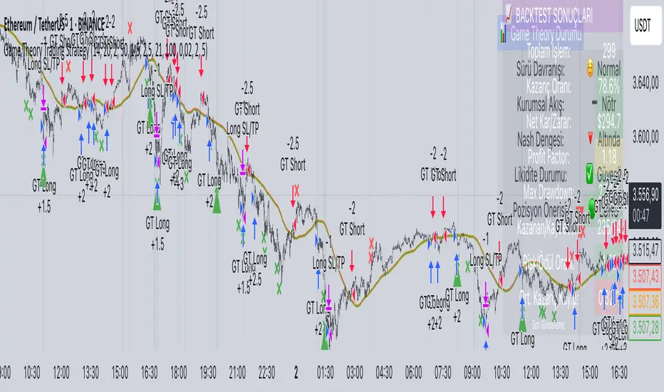
Game Theory Trading StrategyGame Theory Trading Strategy: Explanation and Working Logic
This Pine Script (version 5) code implements a trading strategy named "Game Theory Trading Strategy" in TradingView. Unlike the previous indicator, this is a full-fledged strategy with automated entry/exit rules, risk management, and backtesting capabilities. It uses Game Theory principles to analyze market behavior, focusing on herd behavior, institutional flows, liquidity traps, and Nash equilibrium to generate buy (long) and sell (short) signals. Below, I'll explain the strategy's purpose, working logic, key components, and usage tips in detail.
1. General Description
Purpose: The strategy identifies high-probability trading opportunities by combining Game Theory concepts (herd behavior, contrarian signals, Nash equilibrium) with technical analysis (RSI, volume, momentum). It aims to exploit market inefficiencies caused by retail herd behavior, institutional flows, and liquidity traps. The strategy is designed for automated trading with defined risk management (stop-loss/take-profit) and position sizing based on market conditions.
Key Features:
Herd Behavior Detection: Identifies retail panic buying/selling using RSI and volume spikes.
Liquidity Traps: Detects stop-loss hunting zones where price breaks recent highs/lows but reverses.
Institutional Flow Analysis: Tracks high-volume institutional activity via Accumulation/Distribution and volume spikes.
Nash Equilibrium: Uses statistical price bands to assess whether the market is in equilibrium or deviated (overbought/oversold).
Risk Management: Configurable stop-loss (SL) and take-profit (TP) percentages, dynamic position sizing based on Game Theory (minimax principle).
Visualization: Displays Nash bands, signals, background colors, and two tables (Game Theory status and backtest results).
Backtesting: Tracks performance metrics like win rate, profit factor, max drawdown, and Sharpe ratio.
Strategy Settings:
Initial capital: $10,000.
Pyramiding: Up to 3 positions.
Position size: 10% of equity (default_qty_value=10).
Configurable inputs for RSI, volume, liquidity, institutional flow, Nash equilibrium, and risk management.
Warning: This is a strategy, not just an indicator. It executes trades automatically in TradingView's Strategy Tester. Always backtest thoroughly and use proper risk management before live trading.
2. Working Logic (Step by Step)
The strategy processes each bar (candle) to generate signals, manage positions, and update performance metrics. Here's how it works:
a. Input Parameters
The inputs are grouped for clarity:
Herd Behavior (🐑):
RSI Period (14): For overbought/oversold detection.
Volume MA Period (20): To calculate average volume for spike detection.
Herd Threshold (2.0): Volume multiplier for detecting herd activity.
Liquidity Analysis (💧):
Liquidity Lookback (50): Bars to check for recent highs/lows.
Liquidity Sensitivity (1.5): Volume multiplier for trap detection.
Institutional Flow (🏦):
Institutional Volume Multiplier (2.5): For detecting large volume spikes.
Institutional MA Period (21): For Accumulation/Distribution smoothing.
Nash Equilibrium (⚖️):
Nash Period (100): For calculating price mean and standard deviation.
Nash Deviation (0.02): Multiplier for equilibrium bands.
Risk Management (🛡️):
Use Stop-Loss (true): Enables SL at 2% below/above entry price.
Use Take-Profit (true): Enables TP at 5% above/below entry price.
b. Herd Behavior Detection
RSI (14): Checks for extreme conditions:
Overbought: RSI > 70 (potential herd buying).
Oversold: RSI < 30 (potential herd selling).
Volume Spike: Volume > SMA(20) x 2.0 (herd_threshold).
Momentum: Price change over 10 bars (close - close ) compared to its SMA(20).
Herd Signals:
Herd Buying: RSI > 70 + volume spike + positive momentum = Retail buying frenzy (red background).
Herd Selling: RSI < 30 + volume spike + negative momentum = Retail selling panic (green background).
c. Liquidity Trap Detection
Recent Highs/Lows: Calculated over 50 bars (liquidity_lookback).
Psychological Levels: Nearest round numbers (e.g., $100, $110) as potential stop-loss zones.
Trap Conditions:
Up Trap: Price breaks recent high, closes below it, with a volume spike (volume > SMA x 1.5).
Down Trap: Price breaks recent low, closes above it, with a volume spike.
Visualization: Traps are marked with small red/green crosses above/below bars.
d. Institutional Flow Analysis
Volume Check: Volume > SMA(20) x 2.5 (inst_volume_mult) = Institutional activity.
Accumulation/Distribution (AD):
Formula: ((close - low) - (high - close)) / (high - low) * volume, cumulated over time.
Smoothed with SMA(21) (inst_ma_length).
Accumulation: AD > MA + high volume = Institutions buying.
Distribution: AD < MA + high volume = Institutions selling.
Smart Money Index: (close - open) / (high - low) * volume, smoothed with SMA(20). Positive = Smart money buying.
e. Nash Equilibrium
Calculation:
Price mean: SMA(100) (nash_period).
Standard deviation: stdev(100).
Upper Nash: Mean + StdDev x 0.02 (nash_deviation).
Lower Nash: Mean - StdDev x 0.02.
Conditions:
Near Equilibrium: Price between upper and lower Nash bands (stable market).
Above Nash: Price > upper band (overbought, sell potential).
Below Nash: Price < lower band (oversold, buy potential).
Visualization: Orange line (mean), red/green lines (upper/lower bands).
f. Game Theory Signals
The strategy generates three types of signals, combined into long/short triggers:
Contrarian Signals:
Buy: Herd selling + (accumulation or down trap) = Go against retail panic.
Sell: Herd buying + (distribution or up trap).
Momentum Signals:
Buy: Below Nash + positive smart money + no herd buying.
Sell: Above Nash + negative smart money + no herd selling.
Nash Reversion Signals:
Buy: Below Nash + rising close (close > close ) + volume > MA.
Sell: Above Nash + falling close + volume > MA.
Final Signals:
Long Signal: Contrarian buy OR momentum buy OR Nash reversion buy.
Short Signal: Contrarian sell OR momentum sell OR Nash reversion sell.
g. Position Management
Position Sizing (Minimax Principle):
Default: 1.0 (10% of equity).
In Nash equilibrium: Reduced to 0.5 (conservative).
During institutional volume: Increased to 1.5 (aggressive).
Entries:
Long: If long_signal is true and no existing long position (strategy.position_size <= 0).
Short: If short_signal is true and no existing short position (strategy.position_size >= 0).
Exits:
Stop-Loss: If use_sl=true, set at 2% below/above entry price.
Take-Profit: If use_tp=true, set at 5% above/below entry price.
Pyramiding: Up to 3 concurrent positions allowed.
h. Visualization
Nash Bands: Orange (mean), red (upper), green (lower).
Background Colors:
Herd buying: Red (90% transparency).
Herd selling: Green.
Institutional volume: Blue.
Signals:
Contrarian buy/sell: Green/red triangles below/above bars.
Liquidity traps: Red/green crosses above/below bars.
Tables:
Game Theory Table (Top-Right):
Herd Behavior: Buying frenzy, selling panic, or normal.
Institutional Flow: Accumulation, distribution, or neutral.
Nash Equilibrium: In equilibrium, above, or below.
Liquidity Status: Trap detected or safe.
Position Suggestion: Long (green), Short (red), or Wait (gray).
Backtest Table (Bottom-Right):
Total Trades: Number of closed trades.
Win Rate: Percentage of winning trades.
Net Profit/Loss: In USD, colored green/red.
Profit Factor: Gross profit / gross loss.
Max Drawdown: Peak-to-trough equity drop (%).
Win/Loss Trades: Number of winning/losing trades.
Risk/Reward Ratio: Simplified Sharpe ratio (returns / drawdown).
Avg Win/Loss Ratio: Average win per trade / average loss per trade.
Last Update: Current time.
i. Backtesting Metrics
Tracks:
Total trades, winning/losing trades.
Win rate (%).
Net profit ($).
Profit factor (gross profit / gross loss).
Max drawdown (%).
Simplified Sharpe ratio (returns / drawdown).
Average win/loss ratio.
Updates metrics on each closed trade.
Displays a label on the last bar with backtest period, total trades, win rate, and net profit.
j. Alerts
No explicit alertconditions defined, but you can add them for long_signal and short_signal (e.g., alertcondition(long_signal, "GT Long Entry", "Long Signal Detected!")).
Use TradingView's alert system with Strategy Tester outputs.
3. Usage Tips
Timeframe: Best for H1-D1 timeframes. Shorter frames (M1-M15) may produce noisy signals.
Settings:
Risk Management: Adjust sl_percent (e.g., 1% for volatile markets) and tp_percent (e.g., 3% for scalping).
Herd Threshold: Increase to 2.5 for stricter herd detection in choppy markets.
Liquidity Lookback: Reduce to 20 for faster markets (e.g., crypto).
Nash Period: Increase to 200 for longer-term analysis.
Backtesting:
Use TradingView's Strategy Tester to evaluate performance.
Check win rate (>50%), profit factor (>1.5), and max drawdown (<20%) for viability.
Test on different assets/timeframes to ensure robustness.
Live Trading:
Start with a demo account.
Combine with other indicators (e.g., EMAs, support/resistance) for confirmation.
Monitor liquidity traps and institutional flow for context.
Risk Management:
Always use SL/TP to limit losses.
Adjust position_size for risk tolerance (e.g., 5% of equity for conservative trading).
Avoid over-leveraging (pyramiding=3 can amplify risk).
Troubleshooting:
If no trades are executed, check signal conditions (e.g., lower herd_threshold or liquidity_sensitivity).
Ensure sufficient historical data for Nash and liquidity calculations.
If tables overlap, adjust position.top_right/bottom_right coordinates.
4. Key Differences from the Previous Indicator
Indicator vs. Strategy: The previous code was an indicator (VP + Game Theory Integrated Strategy) focused on visualization and alerts. This is a strategy with automated entries/exits and backtesting.
Volume Profile: Absent in this strategy, making it lighter but less focused on high-volume zones.
Wick Analysis: Not included here, unlike the previous indicator's heavy reliance on wick patterns.
Backtesting: This strategy includes detailed performance metrics and a backtest table, absent in the indicator.
Simpler Signals: Focuses on Game Theory signals (contrarian, momentum, Nash reversion) without the "Power/Ultra Power" hierarchy.
Risk Management: Explicit SL/TP and dynamic position sizing, not present in the indicator.
5. Conclusion
The "Game Theory Trading Strategy" is a sophisticated system leveraging herd behavior, institutional flows, liquidity traps, and Nash equilibrium to trade market inefficiencies. It’s designed for traders who understand Game Theory principles and want automated execution with robust risk management. However, it requires thorough backtesting and parameter optimization for specific markets (e.g., forex, crypto, stocks). The backtest table and visual aids make it easy to monitor performance, but always combine with other analysis tools and proper capital management.
If you need help with backtesting, adding alerts, or optimizing parameters, let me know!
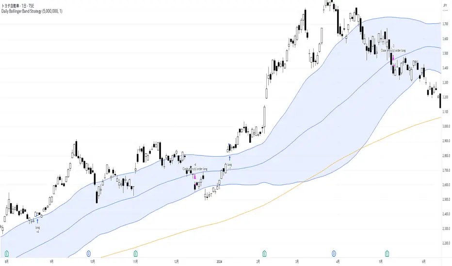
Daily Bollinger Band StrategyOverview of the Daily Bollinger Band Strategy
1. Strategy Overview and Features
This strategy is a tool for backtesting a trading method that uses Bollinger Bands. It is *not* a tool for automated trading.
1-1. Main Display Items
The main chart displays the Bollinger Bands and the 200-day moving average.
It also shows the entry and exit points along with the position size (in units of 100 shares).
1-2. Summary of Trading Rules
For long (buy) strategies, the trade enters when the price crosses above the +1σ line of the Bollinger Bands, aiming to ride an upward trend. The position is exited when the price crosses below the middle band.
For short (sell) strategies, the trade enters when the price crosses below the -1σ line of the Bollinger Bands, aiming to ride a downward trend. The position is exited when the price crosses above the middle band.
1-3. Strategic Enhancements
The strategy uses the slope of the 200-day moving average to determine the trend direction and enter trades accordingly. This improves the win rate and payoff ratio.
Additionally, to reduce the probability of ruin, the risk per trade is limited to 1.0% of capital, and position sizing is adjusted using ATR (a volatility indicator).
2. Trading Rules
2-1. Chart Type
Only daily charts are used.
2-2. Indicators Used
(1) Bollinger Bands** (used for entry and exit signals)
- Period: Fixed at 80 days
- Upper and lower bands: Fixed at ±1σ
(2) Moving Average** (used to determine trend direction)
- Period: Fixed at 200 days
- Trend direction is judged based on whether the difference from the previous day is positive (upward) or negative (downward)
2-3. Buy Rules
Setup:
- Price crosses above the +1σ line from below
- Both the middle band and 200-day moving average are upward sloping
Entry:
- Buy at the next day’s market open using a market order
Exit:
- If the price crosses below the middle band, sell at the next day’s open using a market order
2-4. Sell Rules
Setup:
- Price crosses below the -1σ line from above
- Both the middle band and 200-day moving average are downward sloping
Entry:
- Sell at the next day’s market open using a market order
Exit:
- If the price crosses above the middle band, buy back at the next day’s open using a market order
2-5. Risk Management Rules
- Risk per trade: 1.0% of total capital (acceptable loss = capital × 1.0%)
- Position size: Acceptable loss ÷ 2ATR (rounded down to the nearest unit of 100 shares)
2-6. Other Notes
- No brokerage fees
- No pyramiding
- No partial exits
- No reverse positions (no “stop-and-reverse” trades)
3. Strategy Parameters
The following settings can be specified:
3-1. Period Settings
- Start date: Set the start date for the backtest period
- Stop date: Set the end date for the backtest period
3-2. Display of Trend and Signals
- Show trend: When checked, the background color of the bars is light red for an uptrend and light blue for a downtrend
- Show signal: When checked, entry and exit signals are displayed (note: signals are executed at the next day’s open, so there is a one-day lag in the display)
3-3. Capital Management Settings
- Funds: Capital available for trading (in JPY)
- Risk rate: Specify what percentage of the capital to risk per trade
Settings in the “Properties” tab are not used in this strategy.
4. Backtest Results (Example)
Here are the backtest results conducted by the author:
- Target Stocks: All components of the Nikkei 225
- Test Period: January 4, 2000 – December 30, 2024
- Data Points: 12,886
- Win Rate: 33.45%
- Net Profit: ¥82,132,380
- Payoff Ratio: 2.450
- Expected Value: ¥6,373.8
- Risk Rate: 1.0%
- Probability of Ruin: 0.00%
---
デイリー・ボリンジャーバンド・ストラテジーの概要
1. ストラテジーの概要と特徴
このストラテジーは、ボリンジャーバンドを使ったトレード手法のバックテストを行うツールです。自動売買を行うツールではありません。
1-1. 主な表示項目
メインチャートにボリンジャーバンドと 200日移動平均線を表示します。
また、エントリーと手仕舞いのタイミングと数量(100株単位)も表示されます。
1-2. トレードルールの概要
買い戦略の場合、ボリンジャーバンドの +1σ 超えでエントリーして上昇トレンドに乗り、ミドルバンドを割ったら決済します。
売り戦略の場合、ボリンジャーバンドの -1σ 割りでエントリーして下降トレンドに乗り、ミドルバンドを上抜けたら決済します。
1-3. ストラテジーの工夫点
200日移動平均線の傾きを見てトレンド方向にエントリーをしています。こうして勝率とペイオフレシオの成績を向上しています。
また、破産確率を抑えるために、リスク資金比率を 1.0% にして、ATR(ボラティリティ指標) を使って注文数を調整しています。
2. 売買ルール
2-1. 使用するチャート
日足チャートに限定します
2-2. 使用する指標
(1) ボリンジャーバンド(仕掛けと手仕舞いのシグナルに使用)
期間は80日に固定
上下バンドは ±1σ に固定
(2) 移動平均線(トレンドの方向を見るために使用)
期間は200日に固定
移動平均の値の前日との差がプラスのとき上向き、マイナスのとき下向きと判断
2-3. 買いのルール
セットアップ:ボリンジャーバンドの +1σ を価格が下から上に交差 かつ ミドルバンドと 200日移動平均線が上向き
仕掛け:翌日の寄り付きに成行で買う
手仕舞い:ボリンジャーバンドのミドルバンドを価格が上から下に交差したら、翌日の寄り付きに成行で売る
2-4. 売りのルール
セットアップ:ボリンジャーバンドの -1σ を価格が上から下に交差 かつ ミドルバンドと 200日移動平均線が下向き
仕掛け:翌日の寄り付きに成行で売る
手仕舞い:ボリンジャーバンドのミドルバンドを価格が下から上に交差したら、翌日の寄り付きに成行で買い戻す
2-5. 資金管理のルール
リスク資金比率:資産の 1.0%(許容損失 = 資産 × 1.0%)
注文数:許容損失 ÷ 2ATR(単元株数未満は切り捨て)
2-6. その他
仲介手数料:なし
ピラミッディング:なし
分割決済:なし
ドテン:しない
3. ストラテジーのパラメーター
次の項目が指定できます。
3-1. 期間の設定
Staer date : バックテストの検証期間の開始日を指定します
Stop date : バックテストの検証期間の終了日を指定します
3-2. トレンドとシグナルの表示
Show trend : チェックを入れると、バーの背景色が、トレンドが上昇のときは薄い赤で、下落のときは薄い青で表示されます
Show signal : チェックを入れると、エントリーと手仕舞いのシグナルを表示します(シグナルの出た翌日の寄り付きに売買をするので表示に1日のずれがあります)
3-3. 資金管理用の設定
Funds : トレード用の資金(円)
Risk rate : 許容損失を資金の何%にするかで指定します
「プロパティタブ」で設定する値は、このストラテジーでは有効ではありません。
4. バックテストの結果(例)
作者がバックテストを実施した結果をお知らせします。
対象銘柄:日経225構成銘柄すべて
対象期間:2000年1月4日~2024年12月30日
データ件数:12,886
勝率:33.45%
純利益:82,132,380
ペイオフレシオ:2.450
期待値:6,373.8
リスク資金比率:1.0%
破産確率:0.00%
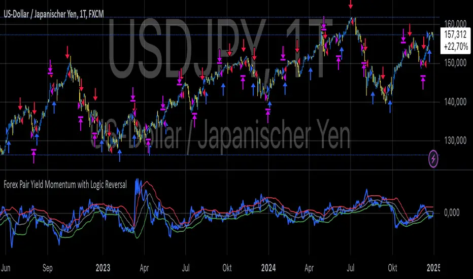
Forex Pair Yield Momentum This Pine Script strategy leverages yield differentials between the 2-year government bond yields of two countries to trade Forex pairs. Yield spreads are widely regarded as a fundamental driver of currency movements, as highlighted by international finance theories like the Interest Rate Parity (IRP), which suggests that currencies with higher yields tend to appreciate due to increased capital flows:
1. Dynamic Yield Spread Calculation:
• The strategy dynamically calculates the yield spread (yield_a - yield_b) for the chosen Forex pair.
• Example: For GBP/USD, the spread equals US 2Y Yield - UK 2Y Yield.
2. Momentum Analysis via Bollinger Bands:
• Yield momentum is computed as the difference between the current spread and its moving
Bollinger Bands are applied to identify extreme deviations:
• Long Entry: When momentum crosses below the lower band.
• Short Entry: When momentum crosses above the upper band.
3. Reversal Logic:
• An optional checkbox reverses the trading logic, allowing long trades at the upper band and short trades at the lower band, accommodating different market conditions.
4. Trade Management:
• Positions are held for a predefined number of bars (hold_periods), and each trade uses a fixed contract size of 100 with a starting capital of $20,000.
Theoretical Basis:
1. Yield Differentials and Currency Movements:
• Empirical studies, such as Clarida et al. (2009), confirm that interest rate differentials significantly impact exchange rate dynamics, especially in carry trade strategies .
• Higher-yields tend to appreciate against lower-yielding currencies due to speculative flows and demand for higher returns.
2. Bollinger Bands for Momentum:
• Bollinger Bands effectively capture deviations in yield momentum, identifying opportunities where price returns to equilibrium (mean reversion) or extends in trend-following scenarios (momentum breakout).
• As Bollinger (2001) emphasized, this tool adapts to market volatility by dynamically adjusting thresholds .
References:
1. Dornbusch, R. (1976). Expectations and Exchange Rate Dynamics. Journal of Political Economy.
2. Obstfeld, M., & Rogoff, K. (1996). Foundations of International Macroeconomics.
3. Clarida, R., Davis, J., & Pedersen, N. (2009). Currency Carry Trade Regimes. NBER.
4. Bollinger, J. (2001). Bollinger on Bollinger Bands.
5. Mendelsohn, L. B. (2006). Forex Trading Using Intermarket Analysis.
Prop Firm Business SimulatorThe prop firm business simulator is exactly what it sounds like. It's a plug and play tool to test out any tradingview strategy and simulate hypothetical performance on CFD Prop Firms.
Now what is a modern day CFD Prop Firm?
These companies sell simulated trading challenges for a challenge fee. If you complete the challenge you get access to simulated capital and you get a portion of the profits you make on those accounts payed out.
I've included some popular firms in the code as presets so it's easy to simulate them. Take into account that this info will likely be out of date soon as these prices and challenge conditions change.
Also, this tool will never be able to 100% simulate prop firm conditions and all their rules. All I aim to do with this tool is provide estimations.
Now why is this tool helpful?
Most traders on here want to turn their passion into their full-time career, prop firms have lately been the buzz in the trading community and market themselves as a faster way to reach that goal.
While this all sounds great on paper, it is sometimes hard to estimate how much money you will have to burn on challenge fees and set realistic monthly payout expectations for yourself and your trading. This is where this tool comes in.
I've specifically developed this for traders that want to treat prop firms as a business. And as a business you want to know your monthly costs and income depending on the trading strategy and prop firm challenge you are using.
How to use this tool
It's quite simple you remove the top part of the script and replace it with your own strategy. Make sure it's written in same version of pinescript before you do that.
//--$$$$$$$$$$$$$$$$$$$$$$$$$$$$$$$$$$$$$$$$$$$$$$$$--//--------------------------------------------------------------------------------------------------------------------------$$$$$$
//--$$$$$--Strategy-- --$$$$$$--// ******************************************************************************************************************************
//--$$$$$$$$$$$$$$$$$$$$$$$$$$$$$$$$$$$$$$$$$$$$$$$$--//--------------------------------------------------------------------------------------------------------------------------$$$$$$
length = input.int(20, minval=1, group="Keltner Channel Breakout")
mult = input(2.0, "Multiplier", group="Keltner Channel Breakout")
src = input(close, title="Source", group="Keltner Channel Breakout")
exp = input(true, "Use Exponential MA", display = display.data_window, group="Keltner Channel Breakout")
BandsStyle = input.string("Average True Range", options = , title="Bands Style", display = display.data_window, group="Keltner Channel Breakout")
atrlength = input(10, "ATR Length", display = display.data_window, group="Keltner Channel Breakout")
esma(source, length)=>
s = ta.sma(source, length)
e = ta.ema(source, length)
exp ? e : s
ma = esma(src, length)
rangema = BandsStyle == "True Range" ? ta.tr(true) : BandsStyle == "Average True Range" ? ta.atr(atrlength) : ta.rma(high - low, length)
upper = ma + rangema * mult
lower = ma - rangema * mult
//--Graphical Display--// *-*-*-*-*-*-*-*-*-*-*-*-*-*-*-*-*-*-*-*-*-*-*-*-*-*-*-*-*-*-*-*-*-*-*-*-*-*-*-*-*-*-*-*-*-*-*-*-*-*-*-*-*-*-*-*-*-*-*-*-*-*-*-*-*-*-*-*-*-*-*-*-*-$$$$$$
u = plot(upper, color=#2962FF, title="Upper", force_overlay=true)
plot(ma, color=#2962FF, title="Basis", force_overlay=true)
l = plot(lower, color=#2962FF, title="Lower", force_overlay=true)
fill(u, l, color=color.rgb(33, 150, 243, 95), title="Background")
//--Risk Management--// *-*-*-*-*-*-*-*-*-*-*-*-*-*-*-*-*-*-*-*-*-*-*-*-*-*-*-*-*-*-*-*-*-*-*-*-*-*-*-*-*-*-*-*-*-*-*-*-*-*-*-*-*-*-*-*-*-*-*-*-*-*-*-*-*-*-*-*-*-*-*-*-*-*-$$$$$$
riskPerTradePerc = input.float(1, title="Risk per trade (%)", group="Keltner Channel Breakout")
le = high>upper ? false : true
se = lowlower
strategy.entry('PivRevLE', strategy.long, comment = 'PivRevLE', stop = upper, qty=riskToLots)
if se and upper>lower
strategy.entry('PivRevSE', strategy.short, comment = 'PivRevSE', stop = lower, qty=riskToLots)
The tool will then use the strategy equity of your own strategy and use this to simulat prop firms. Since these CFD prop firms work with different phases and payouts the indicator will simulate the gains until target or max drawdown / daily drawdown limit gets reached. If it reaches target it will go to the next phase and keep on doing that until it fails a challenge.
If in one of the phases there is a reward for completing, like a payout, refund, extra it will add this to the gains.
If you fail the challenge by reaching max drawdown or daily drawdown limit it will substract the challenge fee from the gains.
These gains are then visualised in the calendar so you can get an idea of yearly / monthly gains of the backtest. Remember, it is just a backtest so no guarantees of future income.
The bottom pane (non-overlay) is visualising the performance of the backtest during the phases. This way u can check if it is realistic. For instance if it only takes 1 bar on chart to reach target you are probably risking more than the firm wants you to risk. Also, it becomes much less clear if daily drawdown got hit in those high risk strategies, the results will be less accurate.
The daily drawdown limit get's reset every time there is a new dayofweek on chart.
If you set your prop firm preset setting to "'custom" the settings below that are applied as your prop firm settings. Otherwise it will use one of the template by default it's FTMO 100K.
The strategy I'm using as an example in this script is a simple Keltner Channel breakout strategy. I'm using a 0.05% commission per trade as that is what I found most common on crypto exchanges and it's close to the commissions+spread you get on a cfd prop firm. I'm targeting a 1% risk per trade in the backtest to try and stay within prop firm boundaries of max 1% risk per trade.
Lastly, the original yearly and monthly performance table was developed by Quantnomad and I've build ontop of that code. Here's a link to the original publication:
That's everything for now, hope this indicator helps people visualise the potential of prop firms better or to understand that they are not a good fit for their current financial situation.
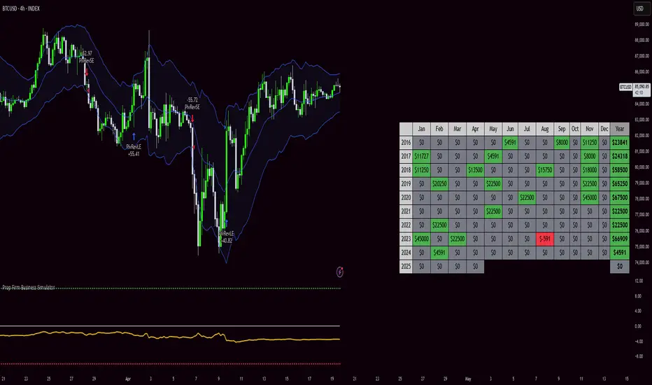
Zero-Lag MA Trend FollowingScript Name: Zero-Lag MA Trend Following Auto-Trading
Purpose and Unique Features:
This script is designed to implement a trend-following auto-trading strategy by combining the Zero-Lag Moving Average (ZLMA), Exponential Moving Average (EMA), and ATR Bands. To differentiate it from similar scripts, the following key aspects are emphasized:
Zero-Lag MA (ZLMA):
Responds quickly to price changes, minimizing lag compared to EMA.
Detects crossovers with EMA and generates Diamond Signals to indicate trend reversals.
ATR Bands:
Measures market volatility to set stop-loss levels.
Helps optimize entry points and manage risk effectively.
Diamond Signals:
A vital visual cue indicating the early stages of trend reversals.
Green diamonds signal an uptrend, while red diamonds signal a downtrend.
Each component plays a distinct role, working synergistically to enhance trend detection and risk management. This system doesn’t merely combine indicators but optimizes them for comprehensive trend-following and risk control.
Usage Instructions:
Entry Conditions:
Long Entry:
Enter when a green Diamond Signal appears (ZLMA crosses above EMA).
Short Entry:
Enter when a red Diamond Signal appears (ZLMA crosses below EMA).
Exit Conditions:
Stop Loss:
Set at the lower boundary of the ATR band for BUY or the upper boundary for SELL at entry.
Take Profit:
Automatically executed based on a 1:2 risk-reward ratio.
Account Size: ¥100,0000
Commissions and Slippage: Assumed commission of 90 pips per trade and slippage of 1 pip.
Risk per Trade: 10% of account equity (adjustable based on risk tolerance).
Improvements and Original Features:
While based on open-source code, this script incorporates the following critical enhancements:
Diamond Signals from ZLMA and EMA Integration:
Improves entry accuracy with a proprietary trend detection strategy.
ATR Bands Utilization:
Adds a volatility-based risk management function.
Optimized Visual Entry Signals:
Includes plotted triangles (▲, ▼) to clearly indicate trend-following entry points.
Credits:
This script builds upon indicators developed by ChartPrime, whose innovative approach and insights have enabled a more advanced trend-following strategy. We extend our gratitude for their foundational work.
Additionally, it integrates technical methods based on Zero-Lag Moving Average (ZLMA), EMA, and ATR Bands, leveraging insights from the trading community.
Chart Display Options:
The script offers options to toggle the visual signals (Diamond Signals, trend lines, and entry points) on or off, keeping the chart clean while maximizing analytical efficiency.
Disclaimer:
This script is provided for educational purposes and past performance does not guarantee future results.
Use it responsibly with proper risk management.

VIDYA Auto-Trading(Reversal Logic)Overview
This script is a dynamic trend-following strategy based on the Variable Index Dynamic Average (VIDYA). It adapts in real time to market volatility, aiming to enhance entry precision and optimize risk management.
⚠️ This strategy is intended for educational and research purposes. Past performance does not guarantee future results. All results are based on historical simulations using fixed parameters.
Strategy Objectives
The objective of this strategy is to respond swiftly to sudden price movements and trend reversals, providing consistent and reliable trade signals under historical testing conditions. It is designed to be intuitive and efficient for traders of all levels.
Key Features
Momentum Sensitivity via VIDYA: Reacts quickly to momentum shifts, allowing for accurate trend-following entries.
Volatility-Based ATR Bands: Automatically adjusts stop levels and entry conditions based on current market volatility.
Intuitive Trend Visualization: Uptrends are marked with green zones, and downtrends with red zones, giving traders clear visual guidance.
Trading Rules
Long Entry: Triggered when price crosses above the upper band. Any existing short position is closed.
Short Entry: Triggered when price crosses below the lower band. Any existing long position is closed.
Exit Conditions: Positions are reversed based on signal changes, using a position reversal strategy.
Risk Management Parameters
Market: ETHUSD(5M)
Account Size: $3,000 (reasonable approximation for individual traders)
Commission: 0.02%
Slippage: 2 pip
Risk per Trade: 5% of account equity (adjusted to comply with TradingView guidelines for realistic risk levels)
Number of Trades: 251 (based on backtest over the selected dataset)
⚠️ The risk per trade and other values can be customized. Users are encouraged to adapt these to their individual needs and broker conditions.
Trading Parameters & Considerations
VIDYA Length: 10
VIDYA Momentum: 20
Distance factor for upper/lower bands: 2
Source: close
Visual Support
Trend zones, entry points, and directional shifts are clearly plotted on the chart. These visual cues enhance the analytical experience and support faster decision-making.
Visual elements are designed to improve interpretability and are not intended as financial advice or trade signals.
Strategy Improvements & Uniqueness
Inspired by the public work of BigBeluga, this script evolves the original concept with meaningful enhancements. By combining VIDYA and ATR bands, it offers greater adaptability and practical value compared to conventional trend-following strategies.
This adaptation is original work and not a direct copy. Improvements are designed to enhance usability, risk control, and market responsiveness.
Summary
This strategy offers a responsive and adaptive approach to trend trading, built on momentum detection and volatility-adjusted risk management. It balances clarity, precision, and practicality—making it a powerful tool for traders seeking reliable trend signals.
⚠️ All results are based on historical data and are subject to change under different market conditions. This script does not guarantee profit and should be used with caution and proper risk management.
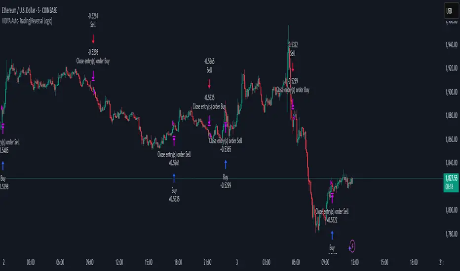
BB Breakout + Momentum Squeeze [Strategy]This Strategy is Based on 3 free indicators
- Bollinger Bands Breakout Oscillator: Link
- TTM Squeeze Pro: Link
- Rolling ATR Bands: Link
Bollinger Bands Breakout Oscillator - This tool shows how strong a market trend is by measuring how often prices move outside their normal Bollinger bands range. It helps you see whether prices are strongly moving in one direction or just moving sideways. By looking at how much and how frequently prices push beyond their typical boundaries, you can identify which direction the market is heading over your selected time period.
TM Squeeze Pro - This is a custom version of the TTM Squeeze indicator.
It's designed to help traders spot consolidation phases in the market (when price is coiling or "squeezing") and to catch breakouts early when volatility returns. The logic is based on the relationship between Bollinger Bands and Keltner Channels, combined with a momentum oscillator to show direction and strength.
Rolling ATR Bands - This indicator combines volatility bands (ATR) with momentum and trend signals to show where the market might be breaking out, retesting, or trending. It's highly visual and helpful for traders looking to time entries/exits during trending or volatile moves.
Logic Of the Strategy:
We are going to use the Bollinger Bands Breakout to determine the direction of the market. Than check the Volatility of the price by looking at the TTM Squeeze indicator. And use the ATR Bands to determine dynamic Stop Losses and based on the calculate the Take Profit targets and quantity for each position dynamically.
For the Long Setup:
1. We need to see the that Bull Power (Green line of the Bollinger Bands Breakout Oscilator) is crossing the level of 50.
2. Check the presence of volatility (Green dot based on the TTM Squeeze indicator)
For the Short Setup:
1. We need to see the that Bear Power (Red line of the Bollinger Bands Breakout Oscilator) is crossing the level of 50.
2. Check the presence of volatility (Green dot based on the TTM Squeeze indicator)
Stop Loss is determined by the Lower ATR Band (for the Long entry) and Upper ATR Band (For the Short entry)
Take Profit is 1:1.5 risk reward ration, which means if the Stop loss is 1% the TP target will be 1.5%
Move stop Loss to Breakeven: If the price will go in the direction of the trade for at least half of the Risk Reward target then the stop will automatically be adjusted to the entry price. For Example: the Stop Loss is 1%, the price has move at least 0.5% in the direction of your trade and that will move the Stop Loss level to the Entry point.
You can Adjust the parameters for each indicator used in that script and also adjust the Risk and Money management block to see how the PnL will change.
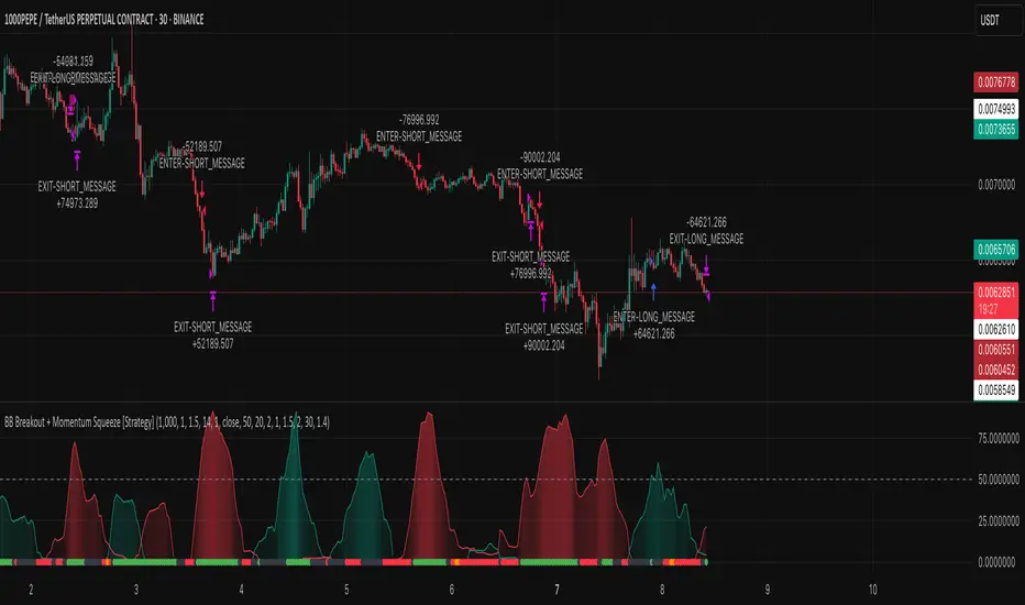
Stochastic-Dynamic Volatility Band ModelThe Stochastic-Dynamic Volatility Band Model is a quantitative trading approach that leverages statistical principles to model market volatility and generate buy and sell signals. The strategy is grounded in the concepts of volatility estimation and dynamic market regimes, where the core idea is to capture price fluctuations through stochastic models and trade around volatility bands.
Volatility Estimation and Band Construction
The volatility bands are constructed using a combination of historical price data and statistical measures, primarily the standard deviation (σ) of price returns, which quantifies the degree of variation in price movements over a specific period. This methodology is based on the classical works of Black-Scholes (1973), which laid the foundation for using volatility as a core component in financial models. Volatility is a crucial determinant of asset pricing and risk, and it plays a pivotal role in this strategy's design.
Entry and Exit Conditions
The entry conditions are based on the price’s relationship with the volatility bands. A long entry is triggered when the price crosses above the lower volatility band, indicating that the market may have been oversold or is experiencing a reversal to the upside. Conversely, a short entry is triggered when the price crosses below the upper volatility band, suggesting overbought conditions or a potential market downturn.
These entry signals are consistent with the mean reversion theory, which asserts that asset prices tend to revert to their long-term average after deviating from it. According to Poterba and Summers (1988), mean reversion occurs due to overreaction to news or temporary disturbances, leading to price corrections.
The exit condition is based on the number of bars that have elapsed since the entry signal. Specifically, positions are closed after a predefined number of bars, typically set to seven bars, reflecting a short-term trading horizon. This exit mechanism is in line with short-term momentum trading strategies discussed in literature, where traders capitalize on price movements within specific timeframes (Jegadeesh & Titman, 1993).
Market Adaptability
One of the key features of this strategy is its dynamic nature, as it adapts to the changing volatility environment. The volatility bands automatically adjust to market conditions, expanding in periods of high volatility and contracting when volatility decreases. This dynamic adjustment helps the strategy remain robust across different market regimes, as it is capable of identifying both trend-following and mean-reverting opportunities.
This dynamic adaptability is supported by the adaptive market hypothesis (Lo, 2004), which posits that market participants evolve their strategies in response to changing market conditions, akin to the adaptive nature of biological systems.
References:
Black, F., & Scholes, M. (1973). The Pricing of Options and Corporate Liabilities. Journal of Political Economy, 81(3), 637-654.
Bollinger, J. (1980). Bollinger on Bollinger Bands. Wiley.
Jegadeesh, N., & Titman, S. (1993). Returns to Buying Winners and Selling Losers: Implications for Stock Market Efficiency. Journal of Finance, 48(1), 65-91.
Lo, A. W. (2004). The Adaptive Markets Hypothesis: Market Efficiency from an Evolutionary Perspective. Journal of Portfolio Management, 30(5), 15-29.
Poterba, J. M., & Summers, L. H. (1988). Mean Reversion in Stock Prices: Evidence and Implications. Journal of Financial Economics, 22(1), 27-59.
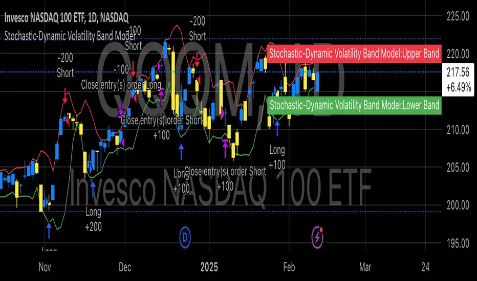
The Bar Counter Trend Reversal Strategy [TradeDots]Overview
The Bar Counter Trend Reversal Strategy is designed to identify potential counter-trend reversal points in the market after a series of consecutive rising or falling bars.
By analyzing price movements in conjunction with optional volume confirmation and channel bands (Bollinger Bands or Keltner Channels), this strategy aims to detect overbought or oversold conditions where a trend reversal may occur.
🔹How it Works
Consecutive Price Movements
Rising Bars: The strategy detects when there are a specified number of consecutive rising bars (No. of Rises).
Falling Bars: Similarly, it identifies a specified number of consecutive falling bars (No. of Falls).
Volume Confirmation (Optional)
When enabled, the strategy checks for increasing volume during the consecutive price movements, adding an extra layer of confirmation to the potential reversal signal.
Channel Confirmation (Optional)
Channel Type: Choose between Bollinger Bands ("BB") or Keltner Channels ("KC").
Channel Interaction: The strategy checks if the price interacts with the upper or lower channel lines: For short signals, it looks for price moving above the upper channel line. For long signals, it looks for price moving below the lower channel line.
Customization:
No. of Rises/Falls: Set the number of consecutive bars required to trigger a signal.
Volume Confirmation: Enable or disable volume as a confirmation factor.
Channel Confirmation: Enable or disable channel bands as a confirmation factor.
Channel Settings: Adjust the length and multiplier for the Bollinger Bands or Keltner Channels.
Visual Indicators:
Entry Signals: Triangles plotted on the chart indicate potential entry points:
Green upward triangle for long entries.
Red downward triangle for short entries.
Channel Bands: The upper and lower bands are plotted for visual reference.
Strategy Parameters:
Initial Capital: $10,000.
Position Sizing: 80% of equity per trade.
Commission: 0.01% per trade to simulate realistic trading costs.
🔹Usage
Set up the number of Rises/Falls and choose whether if you want to use channel indicators and volume as the confirmation.
Monitor the chart for triangles indicating potential entry points.
Consider the context of the overall market trend and other technical factors.
Backtesting and Optimization:
Use TradingView's Strategy Tester to evaluate performance.
Adjust parameters to optimize results for different market conditions.
🔹 Considerations and Recommendations
Risk Management:
The strategy does not include built-in stop-loss or take-profit levels. It's recommended to implement your own risk management techniques.
Market Conditions:
Performance may vary in different market environments. Testing and adjustments are advised when applying the strategy to new instruments or timeframes.
No Guarantee of Future Results:
Past performance is not indicative of future results. Always perform due diligence and consider the risks involved in trading.
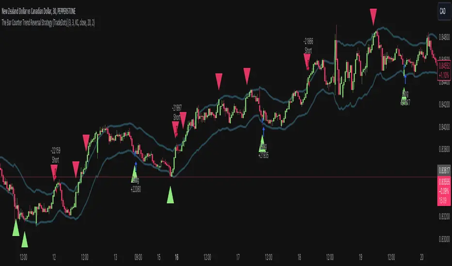
Multi-Step FlexiSuperTrend - Strategy [presentTrading]At the heart of this endeavor is a passion for continuous improvement in the art of trading
█ Introduction and How it is Different
The "Multi-Step FlexiSuperTrend - Strategy " is an advanced trading strategy that integrates the well-known SuperTrend indicator with a nuanced and dynamic approach to market trend analysis. Unlike conventional SuperTrend strategies that rely on static thresholds and fixed parameters, this strategy introduces multi-step take profit mechanisms that allow traders to capitalize on varying market conditions in a more controlled and systematic manner.
What sets this strategy apart is its ability to dynamically adjust to market volatility through the use of an incremental factor applied to the SuperTrend calculation. This adjustment ensures that the strategy remains responsive to both minor and major market shifts, providing a more accurate signal for entries and exits. Additionally, the integration of multi-step take profit levels offers traders the flexibility to scale out of positions, locking in profits progressively as the market moves in their favor.
BTC 6hr Long/Short Performance
█ Strategy, How it Works: Detailed Explanation
The Multi-Step FlexiSuperTrend strategy operates on the foundation of the SuperTrend indicator, but with several enhancements that make it more adaptable to varying market conditions. The key components of this strategy include the SuperTrend Polyfactor Oscillator, a dynamic normalization process, and multi-step take profit levels.
🔶 SuperTrend Polyfactor Oscillator
The SuperTrend Polyfactor Oscillator is the heart of this strategy. It is calculated by applying a series of SuperTrend calculations with varying factors, starting from a defined "Starting Factor" and incrementing by a specified "Increment Factor." The indicator length and the chosen price source (e.g., HLC3, HL2) are inputs to the oscillator.
The SuperTrend formula typically calculates an upper and lower band based on the average true range (ATR) and a multiplier (the factor). These bands determine the trend direction. In the FlexiSuperTrend strategy, the oscillator is enhanced by iteratively applying the SuperTrend calculation across different factors. The iterative process allows the strategy to capture both minor and significant trend changes.
For each iteration (indexed by `i`), the following calculations are performed:
1. ATR Calculation: The Average True Range (ATR) is calculated over the specified `indicatorLength`:
ATR_i = ATR(indicatorLength)
2. Upper and Lower Bands Calculation: The upper and lower bands are calculated using the ATR and the current factor:
Upper Band_i = hl2 + (ATR_i * Factor_i)
Lower Band_i = hl2 - (ATR_i * Factor_i)
Here, `Factor_i` starts from `startingFactor` and is incremented by `incrementFactor` in each iteration.
3. Trend Determination: The trend is determined by comparing the indicator source with the upper and lower bands:
Trend_i = 1 (uptrend) if IndicatorSource > Upper Band_i
Trend_i = 0 (downtrend) if IndicatorSource < Lower Band_i
Otherwise, the trend remains unchanged from the previous value.
4. Output Calculation: The output of each iteration is determined based on the trend:
Output_i = Lower Band_i if Trend_i = 1
Output_i = Upper Band_i if Trend_i = 0
This process is repeated for each iteration (from 0 to 19), creating a series of outputs that reflect different levels of trend sensitivity.
Local
🔶 Normalization Process
To make the oscillator values comparable across different market conditions, the deviations between the indicator source and the SuperTrend outputs are normalized. The normalization method can be one of the following:
1. Max-Min Normalization: The deviations are normalized based on the range of the deviations:
Normalized Value_i = (Deviation_i - Min Deviation) / (Max Deviation - Min Deviation)
2. Absolute Sum Normalization: The deviations are normalized based on the sum of absolute deviations:
Normalized Value_i = Deviation_i / Sum of Absolute Deviations
This normalization ensures that the oscillator values are within a consistent range, facilitating more reliable trend analysis.
For more details:
🔶 Multi-Step Take Profit Mechanism
One of the unique features of this strategy is the multi-step take profit mechanism. This allows traders to lock in profits at multiple levels as the market moves in their favor. The strategy uses three take profit levels, each defined as a percentage increase (for long trades) or decrease (for short trades) from the entry price.
1. First Take Profit Level: Calculated as a percentage increase/decrease from the entry price:
TP_Level1 = Entry Price * (1 + tp_level1 / 100) for long trades
TP_Level1 = Entry Price * (1 - tp_level1 / 100) for short trades
The strategy exits a portion of the position (defined by `tp_percent1`) when this level is reached.
2. Second Take Profit Level: Similar to the first level, but with a higher percentage:
TP_Level2 = Entry Price * (1 + tp_level2 / 100) for long trades
TP_Level2 = Entry Price * (1 - tp_level2 / 100) for short trades
The strategy exits another portion of the position (`tp_percent2`) at this level.
3. Third Take Profit Level: The final take profit level:
TP_Level3 = Entry Price * (1 + tp_level3 / 100) for long trades
TP_Level3 = Entry Price * (1 - tp_level3 / 100) for short trades
The remaining portion of the position (`tp_percent3`) is exited at this level.
This multi-step approach provides a balance between securing profits and allowing the remaining position to benefit from continued favorable market movement.
█ Trade Direction
The strategy allows traders to specify the trade direction through the `tradeDirection` input. The options are:
1. Both: The strategy will take both long and short positions based on the entry signals.
2. Long: The strategy will only take long positions.
3. Short: The strategy will only take short positions.
This flexibility enables traders to tailor the strategy to their market outlook or current trend analysis.
█ Usage
To use the Multi-Step FlexiSuperTrend strategy, traders need to set the input parameters according to their trading style and market conditions. The strategy is designed for versatility, allowing for various market environments, including trending and ranging markets.
Traders can also adjust the multi-step take profit levels and percentages to match their risk management and profit-taking preferences. For example, in highly volatile markets, traders might set wider take profit levels with smaller percentages at each level to capture larger price movements.
The normalization method and the incremental factor can be fine-tuned to adjust the sensitivity of the SuperTrend Polyfactor Oscillator, making the strategy more responsive to minor market shifts or more focused on significant trends.
█ Default Settings
The default settings of the strategy are carefully chosen to provide a balanced approach between risk management and profit potential. Here is a breakdown of the default settings and their effects on performance:
1. Indicator Length (10): This parameter controls the lookback period for the ATR calculation. A shorter length makes the strategy more sensitive to recent price movements, potentially generating more signals. A longer length smooths out the ATR, reducing sensitivity but filtering out noise.
2. Starting Factor (0.618): This is the initial multiplier used in the SuperTrend calculation. A lower starting factor makes the SuperTrend bands closer to the price, generating more frequent trend changes. A higher starting factor places the bands further away, filtering out minor fluctuations.
3. Increment Factor (0.382): This parameter controls how much the factor increases with each iteration of the SuperTrend calculation. A smaller increment factor results in more gradual changes in sensitivity, while a larger increment factor creates a wider range of sensitivity across the iterations.
4. Normalization Method (None): The default is no normalization, meaning the raw deviations are used. Normalization methods like Max-Min or Absolute Sum can make the deviations more consistent across different market conditions, improving the reliability of the oscillator.
5. Take Profit Levels (2%, 8%, 18%): These levels define the thresholds for exiting portions of the position. Lower levels (e.g., 2%) capture smaller profits quickly, while higher levels (e.g., 18%) allow positions to run longer for more significant gains.
6. Take Profit Percentages (30%, 20%, 15%): These percentages determine how much of the position is exited at each take profit level. A higher percentage at the first level locks in more profit early, reducing exposure to market reversals. Lower percentages at higher levels allow for a portion of the position to benefit from extended trends.