Market Regime AnalyzerStatistical regime detection with forward-looking transition probabilities. Combines drift testing, variance ratios, and volume delta to classify markets into 5 regimes and quantify transition probabilities.
What Regime Are We In, and What's Likely Next?
That's the question this indicator answers with statistical rigor and forward-looking probabilities.
The Problem:
Most traders classify regimes arbitrarily: "Bull if price > 200 MA" or "Bear if RSI < 30." These rules ignore statistical significance, volume confirmation, and mean reversion patterns. The result? Late entries, false signals, and confusion when markets transition.
The Solution:
Market Regime Analyzer combines drift detection, variance ratio testing, and volume delta analysis to classify markets into 5 distinct regimes. Then it calculates the probability of transitioning to each regime based on historical patterns.
The Benefit:
Know not just where you are, but where you're likely going - with probabilities, not guesses.
The Five Market Regimes
🟢 Strong Bull (Regime 1)
- Statistically significant upward drift (t-stat > 1.96)
- Strong buying pressure (volume delta > 0.3)
- No mean reversion detected
- **Trade:** Trend-following strategies, ride the momentum
🟢 Weak Bull (Regime 2)
- Upward drift present
- BUT weak volume OR mean reversion detected
- **Trade:** Reduce position size, tighten stops, prepare for consolidation
⚪ Consolidation (Regime 3)
- No statistically significant drift
- Mixed volume signals
- Mean reversion likely present
- **Trade:** Range-trading, avoid trend-following systems
🔴 Weak Bear (Regime 4)
- Downward drift present
- BUT weak volume pressure
- **Trade:** Cautious shorts, reduce exposure, prepare for bounce
🔴 Strong Bear (Regime 5)
- Statistically significant downward drift (t-stat < -1.96)
- Strong selling pressure (volume delta < -0.3)
- No mean reversion detected
- **Trade:** Trend-following shorts, protective puts
The Statistical Framework
1. Drift Detection with T-Statistics
Instead of guessing if there's a trend, we test it statistically.
How it works:
- Calculates mean return over lookback period
- Standardizes by volatility
- Compares to significance threshold (default 1.96 = 95% confidence)
What it tells you:
- T-stat > 1.96: Statistically significant uptrend
- T-stat < -1.96: Statistically significant downtrend
- In between: No significant trend (consolidation)
Why it matters:
Only trades trends that are statistically validated, not just visually apparent.
2. Mean Reversion Testing (Variance Ratio)
Based on Lo & MacKinlay (1988) research, this detects when markets are range-bound.
How it works:
- Compares variance at different time scales
- Variance Ratio < 0.8 indicates mean reversion
What it tells you:
- Mean reversion = NO: Trends can continue
- Mean reversion = YES: Expect price to return to mean, not breakout
Why it matters:
Prevents chasing breakouts in range-bound markets.
3. Volume Delta Analysis
Total volume tells you HOW MUCH traded. Volume delta tells you WHO won.
How it works:
- Buying pressure - Selling pressure = Volume Delta
- Normalized to show relative strength
What it tells you:
- Strong positive delta (>0.3): Buyers in control
- Strong negative delta (<-0.3): Sellers in control
- Weak delta: No clear winner
Why it matters:
Price can move up on weak buying or down on weak selling. Volume delta reveals the truth.
4. Transition Probability Matrix
Historical regime changes predict future regime changes.
How it works:
- Tracks every regime transition over last 100 bars (configurable)
- Builds probability distribution for next regime
- Updates continuously
Example:
Current: Strong Bull
Historical transitions from Strong Bull:
- Stayed Strong Bull: 45%
- Became Weak Bull: 30%
- Became Consolidation: 20%
- Became Weak Bear: 4%
- Became Strong Bear: 1%
What it tells you:
Strong Bull has 75% chance of staying bullish (45% + 30%), only 5% chance of bearish turn.
Why it matters:
Adapts to your specific market's behavior patterns.
How to Use This Indicator
Strategy Adaptation
In Strong Bull/Bear Regimes:
- Use trend-following strategies
- Wider stops, let winners run
- Add to positions on pullbacks
- High confidence in directional trades
In Weak Bull/Bear Regimes:
- Reduce position sizes by 50%
- Tighter stops
- Take profits earlier
- Prepare for regime change
In Consolidation:
- Switch to range-trading strategies
- Avoid trend-following systems
- Sell resistance, buy support
- Wait for regime change before trend trades
Risk Management
Position Sizing:
- Strong regime + high continuation probability (>60%) = Normal size
- Weak regime OR high transition probability = Half size
- Consolidation = Quarter size or skip
Stop Loss Placement:
- Strong regime: Use wider stops (2x ATR)
- Weak regime: Tighter stops (1x ATR)
- Consolidation: Very tight stops (0.5x ATR)
Entry Timing
Best entries:
- Regime just changed to Strong Bull/Bear
- High probability (>50%) of staying in current regime
- No divergence signals present
- Drift and volume delta aligned
Avoid entries:
- High probability of regime change
- Divergence signals appearing
- Mean reversion detected in trending regime
- Weak volume despite price movement
Reading the Dashboard
Current Regime
Color-coded for instant recognition:
- Dark Green = Strong Bull
- Light Green = Weak Bull
- Gray = Consolidation
- Light Red = Weak Bear
- Dark Red = Strong Bear
Annualized Drift
Expected annual return based on recent trend.
- Positive = Upward bias
- Negative = Downward bias
- Near zero = No directional edge
T-Statistic
Measures statistical significance of drift.
- > 1.96 = 95% confident in uptrend
- < -1.96 = 95% confident in downtrend
- Between = Not statistically significant
Mean Reversion
- Yes = Expect price to return to mean (range-bound)
- No = Trends can continue (trending market)
Volume Pressure
Normalized volume delta strength.
- > 0.3 = Strong buying
- < -0.3 = Strong selling
- Near 0 = Balanced
Transition Probabilities
Shows most likely next regime.
- Highest probability = Most likely outcome
- Evenly distributed = High uncertainty
- Concentrated = High confidence in direction
Practical Examples
Example 1: Strong Bull with High Continuation
Dashboard shows:
Current Regime: Strong Bull
Drift: +22% annualized
T-Stat: 3.2
Mean Reversion: No
Volume Pressure: +0.45
Probabilities:
→ Strong Bull: 50%
→ Weak Bull: 25%
→ Consolidation: 20%
→ Bears: 5%
Interpretation:
- Strong uptrend (t-stat 3.2 >> 1.96)
- No mean reversion = trends can continue
- Strong buying pressure (0.45 > 0.3)
- 75% chance stays bullish (50% + 25%)
Action:
- Full position size on long setups
- Use trend-following entries
- Wider stops (2x ATR)
- High conviction trades
Example 2: Weak Bull Before Consolidation
Dashboard shows:
Current Regime: Weak Bull
Drift: +8% annualized
T-Stat: 1.2
Mean Reversion: Yes
Volume Pressure: +0.15
Probabilities:
→ Strong Bull: 10%
→ Weak Bull: 30%
→ Consolidation: 50%
→ Weak Bear: 10%
Interpretation:
- Weak drift (t-stat 1.2 < 1.96)
- Mean reversion detected = range-bound likely
- Weak volume (0.15 < 0.3)
- 50% chance of consolidation
Action:
- Reduce long positions
- Tighten stops
- Prepare for range-bound trading
- Avoid new trend trades
Example 3: Regime Transition Alert
Previous: Weak Bull
Current: Consolidation
Volume divergence signal appeared:
Price made new high, volume delta weakened
Interpretation:
- Trend exhausted
- Buyers losing control
- Regime confirmed the transition
Action:
- Exit trend-following longs
- Switch to range-trading approach
- Wait for new regime before new directional trades
Settings Guide
### Regime Detection Period (50)
Number of bars for statistical calculations.
- **30-40:** More responsive, catches changes faster, more regime switches
- **50 (default):** Balanced for daily/4H charts
- **75-100:** More stable, fewer false regime changes, slower to adapt
Transition History Depth (100)
How much history to use for probabilities.
- **50-75:** Adapts quickly to recent behavior
- **100 (default):** Balanced robustness
- **150-200:** More stable probabilities, slower to adapt
Volume Delta Period (14)
Period for volume calculations.
- **7-10:** More sensitive to volume shifts
- **14 (default):** Standard period
- **20-30:** Smoother, less noise
Significance Threshold (1.96)
T-statistic required for trend classification.
- **1.64:** 90% confidence, more trend regimes detected
- **1.96 (default):** 95% confidence, balanced
- **2.58:** 99% confidence, very conservative, mostly consolidation
Best Practices
Do:
- Wait for regime confirmation (at least 3-5 bars in new regime)
- Use probabilities to size positions appropriately
- Combine with support/resistance for entries
- Respect mean reversion signals
- Adapt strategy to current regime
Don't:
- Trade every regime change immediately
- Ignore high transition probabilities
- Use trend strategies in consolidation
- Override statistical signals with gut feel
- Trade against Strong regimes without clear setup
Timeframe Recommendations
Daily Charts:
- Default settings work well
- Most reliable regime detection
- Best for swing trading
4H Charts:
- Use default or slightly higher lookback (60-75)
- Good for active swing trading
- More regime changes than daily
1H Charts:
- Reduce lookback to 30-40
- More noise, use with caution
- Better for intraday position trading
15M and below:
- Not recommended
- Too much noise for statistical validity
- Regimes change too frequently
Combining with Other Indicators
Works Well With:
Moving Averages
- Use regime for directional bias
- MAs for specific entry/exit points
Support/Resistance
- Regime shows context
- S/R shows specific levels
- High probability at confluence
Volume Profile
- Regime shows regime
- Profile shows where volume is
- Target high-volume nodes
RSI/MACD
- Regime provides context
- Momentum shows entry timing
- Combine for higher probability
Example Combined Setup
Regime: Strong Bull
Price: Above 200 MA
Level: Pullback to support
RSI: Oversold (30)
Volume Delta: Still positive
Setup: Long entry
Reason: Trend intact, healthy pullback, buyers still present
Divergence Signals
The indicator shows volume divergence warnings:
Bearish Divergence (Red Triangle Down)
- Price makes new high
- Volume delta makes lower high
- Warning: Buyers weakening, potential reversal
Bullish Divergence (Green Triangle Up)
- Price makes new low
- Volume delta makes higher low
- Warning: Sellers weakening, potential reversal
How to use:
- Divergence in Strong regime = early warning of regime change
- Confirms when regime actually transitions
- Don't trade divergence alone, wait for regime confirmation
Limitations
This Indicator Cannot:
**Predict black swan events** - Unexpected news overrides all technical regimes
**Work in all markets** - Needs liquid markets with reliable volume data
**Guarantee profits** - Probabilities are not certainties
**Replace fundamental analysis** - Technical regimes can diverge from fundamentals
Works Best:
- Liquid markets (major indices, forex, crypto, large-cap stocks)
- Daily and 4H timeframes
- Combined with other analysis
- With proper risk management
- In normal market conditions
Common Questions
"Why did the regime stay consolidation despite strong price move?"
The indicator detected mean reversion (variance ratio < 0.8), indicating the move will likely reverse. Or the move wasn't statistically significant (t-stat < 1.96). Trust the statistics over visual appearance.
"Probabilities show 30% for each regime. What does that mean?"
High uncertainty. The market is at an inflection point. Reduce position sizes and wait for clearer regime formation.
"Can I use this for day trading?"
Not recommended on timeframes below 1H. Statistical tests need sufficient data. Better suited for swing trading.
"Why does this show Strong Bull when my momentum indicators show weakness?"
Momentum can weaken while the trend remains statistically significant. The indicator focuses on drift and volume, not momentum. Consider it a different perspective.
Technical Notes
Volume Delta Approximation
Uses OHLCV data to approximate order flow:
- Buy volume ≈ Volume on up-closes
- Sell volume ≈ Volume on down-closes
- Delta = Buy - Sell
**Note:** Real order flow (from futures or Level 2) is more precise. This approximation works well on liquid markets.
Statistical Tests
Drift T-Test:
- Null hypothesis: No drift (mean return = 0)
- Reject if |t-stat| > threshold
- Based on standard hypothesis testing
Variance Ratio:
- Compares 2-period variance to 1-period variance
- Ratio = 1 for random walk
- Ratio < 1 for mean reversion
- Threshold of 0.8 based on empirical testing
Transition Probability Implementation
Due to Pine Script v5 limitations (no native 2D arrays), the 5×5 transition matrix is stored as a flat 1D array of 25 elements:
- Position maps to index: `row × 5 + col`
- Example: Transition from Regime 2 to Regime 4 is at index `1 × 5 + 3 = 8`
- Laplace smoothing (0.1) prevents zero probabilities
- Row sums normalized to calculate probabilities
This approach is computationally efficient and maintains statistical accuracy.
No Repainting
All calculations confirmed on bar close. Regime changes appear when the bar closes, not during formation. Historical analysis is accurate.
Alert Conditions
Regime Change
- Triggers when regime transitions to any new state
- Message shows new regime number (1-5)
Bearish Divergence
- Triggers when price makes new high but volume delta doesn't confirm
Bullish Divergence
- Triggers when price makes new low but volume delta doesn't confirm
Disclaimer
FOR EDUCATIONAL PURPOSES ONLY
This indicator uses statistical methods to analyze market regimes. It does not predict the future or guarantee trading success.
Markets are probabilistic, not deterministic. A 70% probability of staying bullish means 30% chance of regime change. Always use proper risk management.
Past regime transitions do not guarantee future transitions. Market structure can change. Statistical relationships can break down.
Never risk more than you can afford to lose. Use stop losses on every trade. Test thoroughly before live trading. Consult a qualified financial advisor.
© 2026 | Open Source
Statistical rigor meets practical application
Statistic

RSquared (log prices)Rolling Trend R² measures the strength of trends using a rolling R² calculation on log prices. Values near 1 indicate a strong, persistent trend, while low values signal choppy or mean-reverting conditions. Includes regime highlighting, reference levels, and an info panel for quick market state identification.

Monte Carlo Simulation BandsMonte Carlo Simulation v2.4.2
Plots a one-bar-ahead price distribution band built from many simulated paths. The green band shows empirical percentiles of simulated final prices—these are distribution bounds, not a confidence interval of the mean.
What It Does
Simulates many one-bar price paths using a directional random walk with volatility scaling (uniform shocks, not Gaussian GBM).
Plots Mean Forecast, Median Forecast, and configurable percentile bounds (default 5th/95th).
Optional rolling HTF-days mean line (yellow) for trend context.
Optional labels and forward projection lines.
Alerts when the confirmed close breaks above or below the percentile band.
Non-Repainting & HTF Behavior (Fail-Closed)
All calculations are gated to confirmed bars only via explicit no_repaint_ok gate (barstate.isconfirmed).
If you select an HTF Resolution, the script uses a strict request.security(..., lookahead_off, gaps_off) pipeline.
If HTF data is unavailable, outputs are na—no silent fallback to chart timeframe.
A separate "HTF Alignment (lagged)" plot shows the prior HTF close (htf_price ) as visual proof of no look-ahead.
Volatility Source & Scaling
If "Use Historical Volatility" is enabled, volatility is estimated from log returns on the selected resolution (HTF if set, otherwise chart).
Annualization adapts to session type:
Equities: 6.5 hours/day, 252 trading days/year
Crypto: 24 hours/day, 365 days/year
Substeps increase path smoothness within the same one-bar horizon—they do not extend the forecast to multiple bars.
Key Inputs
• Prob Up / Prob Down — Must satisfy Prob Up + Prob Down ≤ 1.0. If violated, simulation is skipped and table shows "✗ PROB>1".
• # Simulations / # Substeps — Higher = smoother/more stable, but slower. Default 100×100 is a good balance.
• Lower/Upper Percentile — Define the band width (e.g., 5 and 95 for a 90% distribution band).
• Run On Last Bar Only — Performance mode (recommended). Skips historical computation; updates on each new confirmed bar.
• Resolution (HTF) — Leave blank for chart timeframe, or set to Weekly/Monthly for HTF-aligned simulation.
• Crypto 24/7 Session? — Enable for crypto markets to use correct annualization (365d, 24h).
How to Use (Quickstart)
Start with defaults and keep Run On Last Bar Only = true for speed.
Set Prob Up and Prob Down so their sum ≤ 1.0 (e.g., 0.5 + 0.5 = 1.0 for neutral).
Enable "Use Historical Volatility" and set a Volatility Lookback (e.g., 20 bars) for data-driven vol.
Set Resolution (HTF) if you want the model to run on higher timeframe data (e.g., 1W). Expect updates only when a new HTF interval starts.
Choose percentiles (e.g., 5 and 95) to define your distribution band width.
Enable alerts for "Price Above Upper Percentile" or "Price Below Lower Percentile" to get notified of breakouts.
Limitations & Disclosures
Forecast horizon is one bar only. Substeps do not create a multi-bar forecast.
Model uses uniform shocks with direction chosen from Prob Up/Down. This is not Geometric Brownian Motion (GBM) and is not calibrated to any option-implied distribution.
Bounds are percentiles of final simulated prices, not a statistical confidence interval of the mean.
HTF mode updates at the start of a new HTF interval (first chart bar where the HTF timestamp changes), so the band appears "step-like" in realtime.
Historical volatility requires enough bars for the selected lookback; until then, values may be na.
Performance depends on Sims × Substeps; extreme settings (e.g., 500×500) can be slow.
This indicator does not predict direction—it shows a probabilistic range based on your inputs.

Historical Returns [BigBeluga]🔵 OVERVIEW
The Historical Returns indicator visualizes daily and monthly return data to help traders assess seasonal performance and volatility behavior. It provides a clean and informative dashboard showing the current month’s daily return bubbles, monthly return curves, and a snapshot of the current month and year performance. This tool is ideal for spotting recurring return patterns and understanding the broader profitability context of a symbol.
🔵 CONCEPTS
Daily Return Bubbles: Each trading day is analyzed for its return percentage, and plotted as a bubble with size proportional to the return magnitude.
Monthly Performance Curves: Average or cumulative returns are calculated and plotted to show how the current month is performing relative to historical averages.
Current Year Return: Current year performance as a single return value, giving traders context on long-term profitability.
Current Month Average Return: Current month average performance as a single return value, giving traders context on short-term profitability.
Extreme Return Labels: Optionally highlights daily returns above +4% or below -4% with labeled percentages for spike recognition.
🔵 FEATURES
Shows daily return bubbles (1%–7%+), color-coded by direction.
Labels monthly returns with the month name and percentage value.
Displays a performance dashboard with:
Daily return heatmap for the current month.
Average return for the current month.
Year-to-date return.
Toggle between average and cumulative modes for monthly return curves.
Clearly marks days with abnormal return spikes using optional labels.
Clean fallback warning if not on a daily chart ("⚠️USE DAILY TIMEFRAME").
Custom color themes for bullish and bearish values.
🔵 HOW TO USE
Use the monthly return curve to compare how the current month is performing against historical averages.
Look for clusters of positive or negative bubbles as signals of strong directional weeks.
Watch extreme return labels for volatility spikes or catalyst days.
Use year-to-date return to assess how the asset is trending in the broader macro cycle.
Combine with other BigBeluga tools to align trades with historically favorable periods.
🔵 CONCLUSION
Historical Returns is your visual companion for return analytics — helping you identify profitable months, detect volatility surges, and understand historical seasonality at a glance. With a clean dashboard and insightful overlays, this tool supports better timing and improved statistical edge in both short- and long-term trades.

Stock Relative Strength Rotation Graph🔄 Visualizing Market Rotation & Momentum (Stock RSRG)
This tool visualizes the sector rotation of your watchlist on a single graph. Instead of checking 40 different charts, you can see the entire market cycle in one view. It plots Relative Strength (Trend) vs. Momentum (Velocity) to identify which assets are leading the market and which are lagging.
📜 Credits & Disclaimer
Original Code: Adapted from the open-source " Relative Strength Scatter Plot " by LuxAlgo.
Trademark: This tool is inspired by Relative Rotation Graphs®. Relative Rotation Graphs® is a registered trademark of JOOS Holdings B.V. This script is neither endorsed, nor sponsored, nor affiliated with them.
📊 How It Works (The Math)
The script calculates two metrics for every symbol against a benchmark (Default: SPX):
X-Axis (RS-Ratio): Is the trend stronger than the benchmark? (>100 = Yes)
Y-Axis (RS-Momentum): Is the trend accelerating? (>100 = Yes)
🧩 The 4 Market Quadrants
🟩 Leading (Top-Right): Strong Trend + Accelerating. (Best for holding).
🟦 Improving (Top-Left): Weak Trend + Accelerating. (Best for entries).
⬜ Weakening (Bottom-Right): Strong Trend + Decelerating. (Watch for exits).
🟥 Lagging (Bottom-Left): Weak Trend + Decelerating. (Avoid).
✨ Significant Improvements
This open-source version adds unique features not found in standard rotation scripts:
📝 Quick-Input Engine: Paste up to 40 symbols as a single comma-separated list (e.g., NVDA, AMD, TSLA). No more individual input boxes.
🎯 Quadrant Filtering: You can now hide specific quadrants (like "Lagging") to clear the noise and focus only on actionable setups.
🐛 Trajectory Trails: Visualizes the historical path of the rotation so you can see the direction of momentum.
🛠️ How to Use
Paste Watchlist: Go to settings and paste your symbols (e.g., US Sectors: XLK, XLF, XLE...).
Find Entries: Look for tails moving from Improving ➔ Leading.
Find Exits: Be cautious when tails move from Leading ➔ Weakening.
Zoom: Use the "Scatter Plot Resolution" setting to zoom in or out if dots are bunched up.

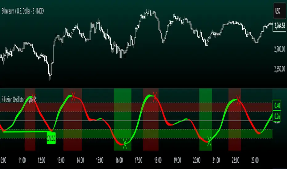
Z-Fusion Oscillator | Lyro RSThe Z-Fusion Oscillator converts five momentum indicators into Z-scores and blends them into one normalized signal that adapts across markets.
By combining normalization, smoothing, and divergence detection, users can easily identify when momentum is accelerating, weakening, reversing, or entering extreme zones
🔶 USAGE
The Z-Fusion Oscillator is designed to give traders a unified reading of market momentum—removing the noise of comparing tools that normally run on different scales.
By transforming RSI, MACD histogram, Stochastic, Momentum, and Rate of Change into Z-scores, this tool standardizes all inputs, making trend strength and shifts easier to interpret.
A dual-line system (fast Z-fusion line + slower baseline) highlights turning points, while overbought/oversold bands and “X-marks” help traders spot exhaustion and potential reversals.
🔹 Unified Momentum Structure
The indicator’s core strength comes from combining five Z-scored signals into one average.
Which makes momentum behavior more consistent across assets, reduces false extremes, and highlights true shifts in trend conviction.
🔹 Divergence Detection
The tool includes fully integrated divergence detection:
Regular Bullish Divergence: Price makes a lower low while Z-Fusion forms a higher low.
Regular Bearish Divergence: Price makes a higher high while Z-Fusion forms a lower high
Bullish and bearish divergences are marked directly on the oscillator with labels and colored pivot connections, making hidden momentum shifts obvious.
🔹 Visual Extremes
Two sets of upper and lower Z-score thresholds help identify:
Extreme overbought surges
Extreme oversold drops
Reversal zones
Potential exhaustion conditions
Background coloring reinforces when the oscillator moves beyond major levels, helping traders quickly assess momentum pressure.
🔹 Detecting Momentum Anomalies
Z-scores allow the oscillator to highlight when market momentum behaves abnormally relative to its own recent history.
For example:
The oscillator reaching +1 or –1 after an extended trend may indicate a climax.
A sharp Z-score reversal within an extreme zone can signal a trend exhaustion or a corrective move.
Divergences often appear earlier due to normalization smoothing out indicator noise.
This makes the Z-Fusion Oscillator particularly useful for spotting subtle shifts in trend direction that traditional indicators may miss.
🔶 DETAILS
🔹 Composite Z-Score Framework
Each momentum tool is smoothed, normalized, and transformed:
RSI → EMA-smoothed, Z-scored
MACD histogram → Z-scored
Stochastic → EMA + SMA smoothing, then Z-scored
Momentum → EMA-smoothed, Z-scored
Rate of Change → EMA-smoothed, Z-scored
These are averaged into one composite Z-score to provide a consistent reading across assets and market conditions.
🔹 Fusion Trend Lines
Two lines serve as the core signal:
Fast Line (savg) – reacts quicker to trend changes
Slow Line (savg2) – acts as a baseline filter
Crossovers between these lines highlight momentum shifts, while their color reflects trend bias.
🔹 Overbought/Oversold Zones
Two upper and two lower Z-score thresholds define “zones”:
Upper zones highlight overheated momentum or potential bearish reversals
Lower zones highlight depressed momentum or potential bullish reversals
Filled regions and background colors help visually confirm extreme conditions.
🔹 Pivot-Based Divergence Engine
The script includes filtered pivot detection with customizable look-backs and range limits to ensure divergences are meaningful, not noise-driven.
🔶 SETTINGS
🔹 Indicator Settings
Source — Price series used for all calculations.
Z-Score Length — Lookback period for Z-score normalization.
Z-Score MA Length — Smoothing length for the fusion signal lines.
Overbought/Oversold Levels — Four customizable threshold lines.
Color Palette — Choose from preset themes or define custom colors.
🔹 RSI
Length — RSI calculation period.
EMA Smoothing Length — Smooths RSI before Z-score conversion.
🔹 MACD
Fast Length — Fast EMA length.
Slow Length — Slow EMA length.
Signal Line Length — MACD signal smoothing.
🔹 Stochastic
%K Length — Main stochastic length.
EMA Smoothing — Smooths %K for stability.
%D Length — Smoothing for the signal line.
🔹 Momentum
Length — Momentum lookback.
EMA Smoothing — Smooths momentum before Z-scoring.
🔹 Rate of Change
Length — ROC lookback.
EMA Smoothing — Smooths ROC values.
🔹 Divergence
Enable/Disable Divergence Detection — Toggle divergence engine.
Pivot Left/Right Lookback — Defines pivot detection sensitivity.
Detection Range Limits — Controls allowable range for divergence.
Bull/Bear Colors & Styling — Customize divergence visualization.
🔶 SUMMARY
The Z-Fusion Oscillator combines multiple momentum signatures into a single normalized signal, enabling traders to:
Identify reversals early
Detect momentum exhaustion
Spot bullish and bearish divergences
Track overbought/oversold conditions
Visualize trend strength with clarity
Whether you're a swing trader, intraday analyst, or trend-reversal hunter, the Z-Fusion Oscillator provides a powerful and adaptive way to read momentum.
Spot-Futures SpreadSpot-Futures Spread Indicator
A comprehensive indicator that automatically calculates and visualizes the percentage spread between spot and perpetual futures prices across multiple exchanges.
Key Features:
Automatic Exchange Detection - Automatically detects your current exchange and finds the corresponding spot/futures pair
Smart Fallback System - If the counterpart isn't available on your exchange, it automatically searches across 7+ major exchanges (Binance, Bybit, OKX, Gate.io, MEXC, KuCoin, HTX) and uses the first valid match
Multi-Exchange Support - Works with 14 exchanges including Binance, Bybit, OKX, MEXC, BitGet, Gate.io, KuCoin, and more
Clear Exchange Attribution - Shows exactly which exchanges are providing spot and futures data in the statistics table
Configurable Moving Average - Track the average spread with customizable period
Standard Deviation Bands - Identify unusual spread conditions with Bollinger-style bands
Built-in Alerts - Get notified when spread crosses bands or zero (parity)
Statistics Table - Real-time stats showing current spread, MA, std dev, and bands
Manual Override Options - Advanced users can manually specify exchanges and symbols
How It Works:
The indicator calculates the spread as: (Futures Price - Spot Price) / Spot Price × 100
Positive spread = Futures trading at a premium (contango)
Negative spread = Futures trading at a discount (backwardation)
Zero = Parity between spot and futures
Use Cases:
Funding Rate Analysis - Correlates with perpetual funding rates
Arbitrage Opportunities - Identify significant spot-futures divergences
Market Sentiment - Premium/discount indicates bullish/bearish positioning
Cross-Exchange Analysis - Compare spreads when spot and futures are on different exchanges
Smart Features:
Works whether you're viewing a spot or futures chart
Automatically handles exchange-specific perpetual contract naming (.P, PERP, SWAP, etc.)
Color-coded visualization (green for premium, red for discount)
Customizable colors and display options
Background shading based on spread direction
Perfect For:
Crypto traders monitoring funding rates, arbitrage traders, market makers, and anyone interested in spot-futures dynamics across multiple exchanges.
Getting Started:
Simply add the indicator to any spot or perpetual futures chart. It will automatically detect the exchange and find the corresponding pair. The statistics table shows which exchanges are being used for maximum transparency.
Note: The indicator automatically ignores invalid symbols, so you'll never see errors even if a specific pair doesn't exist on a particular exchange.
Kudos to @AlekMel that made the "Spot - Fut Spread v2" indicator that I enhance the Automatic detection feature which was not working in some case.

LibWghtLibrary "LibWght"
This is a library of mathematical and statistical functions
designed for quantitative analysis in Pine Script. Its core
principle is the integration of a custom weighting series
(e.g., volume) into a wide array of standard technical
analysis calculations.
Key Capabilities:
1. **Universal Weighting:** All exported functions accept a `weight`
parameter. This allows standard calculations (like moving
averages, RSI, and standard deviation) to be influenced by an
external data series, such as volume or tick count.
2. **Weighted Averages and Indicators:** Includes a comprehensive
collection of weighted functions:
- **Moving Averages:** `wSma`, `wEma`, `wWma`, `wRma` (Wilder's),
`wHma` (Hull), and `wLSma` (Least Squares / Linear Regression).
- **Oscillators & Ranges:** `wRsi`, `wAtr` (Average True Range),
`wTr` (True Range), and `wR` (High-Low Range).
3. **Volatility Decomposition:** Provides functions to decompose
total variance into distinct components for market analysis.
- **Two-Way Decomposition (`wTotVar`):** Separates variance into
**between-bar** (directional) and **within-bar** (noise)
components.
- **Three-Way Decomposition (`wLRTotVar`):** Decomposes variance
relative to a linear regression into **Trend** (explained by
the LR slope), **Residual** (mean-reversion around the
LR line), and **Within-Bar** (noise) components.
- **Local Volatility (`wLRLocTotStdDev`):** Measures the total
"noise" (within-bar + residual) around the trend line.
4. **Weighted Statistics and Regression:** Provides a robust
function for Weighted Linear Regression (`wLinReg`) and a
full suite of related statistical measures:
- **Between-Bar Stats:** `wBtwVar`, `wBtwStdDev`, `wBtwStdErr`.
- **Residual Stats:** `wResVar`, `wResStdDev`, `wResStdErr`.
5. **Fallback Mechanism:** All functions are designed for reliability.
If the total weight over the lookback period is zero (e.g., in
a no-volume period), the algorithms automatically fall back to
their unweighted, uniform-weight equivalents (e.g., `wSma`
becomes a standard `ta.sma`), preventing errors and ensuring
continuous calculation.
---
**DISCLAIMER**
This library is provided "AS IS" and for informational and
educational purposes only. It does not constitute financial,
investment, or trading advice.
The author assumes no liability for any errors, inaccuracies,
or omissions in the code. Using this library to build
trading indicators or strategies is entirely at your own risk.
As a developer using this library, you are solely responsible
for the rigorous testing, validation, and performance of any
scripts you create based on these functions. The author shall
not be held liable for any financial losses incurred directly
or indirectly from the use of this library or any scripts
derived from it.
wSma(source, weight, length)
Weighted Simple Moving Average (linear kernel).
Parameters:
source (float) : series float Data to average.
weight (float) : series float Weight series.
length (int) : series int Look-back length ≥ 1.
Returns: series float Linear-kernel weighted mean; falls back to
the arithmetic mean if Σweight = 0.
wEma(source, weight, length)
Weighted EMA (exponential kernel).
Parameters:
source (float) : series float Data to average.
weight (float) : series float Weight series.
length (simple int) : simple int Look-back length ≥ 1.
Returns: series float Exponential-kernel weighted mean; falls
back to classic EMA if Σweight = 0.
wWma(source, weight, length)
Weighted WMA (linear kernel).
Parameters:
source (float) : series float Data to average.
weight (float) : series float Weight series.
length (int) : series int Look-back length ≥ 1.
Returns: series float Linear-kernel weighted mean; falls back to
classic WMA if Σweight = 0.
wRma(source, weight, length)
Weighted RMA (Wilder kernel, α = 1/len).
Parameters:
source (float) : series float Data to average.
weight (float) : series float Weight series.
length (simple int) : simple int Look-back length ≥ 1.
Returns: series float Wilder-kernel weighted mean; falls back to
classic RMA if Σweight = 0.
wHma(source, weight, length)
Weighted HMA (linear kernel).
Parameters:
source (float) : series float Data to average.
weight (float) : series float Weight series.
length (int) : series int Look-back length ≥ 1.
Returns: series float Linear-kernel weighted mean; falls back to
classic HMA if Σweight = 0.
wRsi(source, weight, length)
Weighted Relative Strength Index.
Parameters:
source (float) : series float Price series.
weight (float) : series float Weight series.
length (simple int) : simple int Look-back length ≥ 1.
Returns: series float Weighted RSI; uniform if Σw = 0.
wAtr(tr, weight, length)
Weighted ATR (Average True Range).
Implemented as WRMA on *true range*.
Parameters:
tr (float) : series float True Range series.
weight (float) : series float Weight series.
length (simple int) : simple int Look-back length ≥ 1.
Returns: series float Weighted ATR; uniform weights if Σw = 0.
wTr(tr, weight, length)
Weighted True Range over a window.
Parameters:
tr (float) : series float True Range series.
weight (float) : series float Weight series.
length (int) : series int Look-back length ≥ 1.
Returns: series float Weighted mean of TR; uniform if Σw = 0.
wR(r, weight, length)
Weighted High-Low Range over a window.
Parameters:
r (float) : series float High-Low per bar.
weight (float) : series float Weight series.
length (int) : series int Look-back length ≥ 1.
Returns: series float Weighted mean of range; uniform if Σw = 0.
wBtwVar(source, weight, length, biased)
Weighted Between Variance (biased/unbiased).
Parameters:
source (float) : series float Data series.
weight (float) : series float Weight series.
length (int) : series int Look-back length ≥ 2.
biased (bool) : series bool true → population (biased); false → sample.
Returns:
variance series float The calculated between-bar variance (σ²btw), either biased or unbiased.
sumW series float The sum of weights over the lookback period (Σw).
sumW2 series float The sum of squared weights over the lookback period (Σw²).
wBtwStdDev(source, weight, length, biased)
Weighted Between Standard Deviation.
Parameters:
source (float) : series float Data series.
weight (float) : series float Weight series.
length (int) : series int Look-back length ≥ 2.
biased (bool) : series bool true → population (biased); false → sample.
Returns: series float σbtw uniform if Σw = 0.
wBtwStdErr(source, weight, length, biased)
Weighted Between Standard Error.
Parameters:
source (float) : series float Data series.
weight (float) : series float Weight series.
length (int) : series int Look-back length ≥ 2.
biased (bool) : series bool true → population (biased); false → sample.
Returns: series float √(σ²btw / N_eff) uniform if Σw = 0.
wTotVar(mu, sigma, weight, length, biased)
Weighted Total Variance (= between-group + within-group).
Useful when each bar represents an aggregate with its own
mean* and pre-estimated σ (e.g., second-level ranges inside a
1-minute bar). Assumes the *weight* series applies to both the
group means and their σ estimates.
Parameters:
mu (float) : series float Group means (e.g., HL2 of 1-second bars).
sigma (float) : series float Pre-estimated σ of each group (same basis).
weight (float) : series float Weight series (volume, ticks, …).
length (int) : series int Look-back length ≥ 2.
biased (bool) : series bool true → population (biased); false → sample.
Returns:
varBtw series float The between-bar variance component (σ²btw).
varWtn series float The within-bar variance component (σ²wtn).
sumW series float The sum of weights over the lookback period (Σw).
sumW2 series float The sum of squared weights over the lookback period (Σw²).
wTotStdDev(mu, sigma, weight, length, biased)
Weighted Total Standard Deviation.
Parameters:
mu (float) : series float Group means (e.g., HL2 of 1-second bars).
sigma (float) : series float Pre-estimated σ of each group (same basis).
weight (float) : series float Weight series (volume, ticks, …).
length (int) : series int Look-back length ≥ 2.
biased (bool) : series bool true → population (biased); false → sample.
Returns: series float σtot.
wTotStdErr(mu, sigma, weight, length, biased)
Weighted Total Standard Error.
SE = √( total variance / N_eff ) with the same effective sample
size logic as `wster()`.
Parameters:
mu (float) : series float Group means (e.g., HL2 of 1-second bars).
sigma (float) : series float Pre-estimated σ of each group (same basis).
weight (float) : series float Weight series (volume, ticks, …).
length (int) : series int Look-back length ≥ 2.
biased (bool) : series bool true → population (biased); false → sample.
Returns: series float √(σ²tot / N_eff).
wLinReg(source, weight, length)
Weighted Linear Regression.
Parameters:
source (float) : series float Data series.
weight (float) : series float Weight series.
length (int) : series int Look-back length ≥ 2.
Returns:
mid series float The estimated value of the regression line at the most recent bar.
slope series float The slope of the regression line.
intercept series float The intercept of the regression line.
wResVar(source, weight, midLine, slope, length, biased)
Weighted Residual Variance.
linear regression – optionally biased (population) or
unbiased (sample).
Parameters:
source (float) : series float Data series.
weight (float) : series float Weighting series (volume, etc.).
midLine (float) : series float Regression value at the last bar.
slope (float) : series float Slope per bar.
length (int) : series int Look-back length ≥ 2.
biased (bool) : series bool true → population variance (σ²_P), denominator ≈ N_eff.
false → sample variance (σ²_S), denominator ≈ N_eff - 2.
(Adjusts for 2 degrees of freedom lost to the regression).
Returns:
variance series float The calculated residual variance (σ²res), either biased or unbiased.
sumW series float The sum of weights over the lookback period (Σw).
sumW2 series float The sum of squared weights over the lookback period (Σw²).
wResStdDev(source, weight, midLine, slope, length, biased)
Weighted Residual Standard Deviation.
Parameters:
source (float) : series float Data series.
weight (float) : series float Weight series.
midLine (float) : series float Regression value at the last bar.
slope (float) : series float Slope per bar.
length (int) : series int Look-back length ≥ 2.
biased (bool) : series bool true → population (biased); false → sample.
Returns: series float σres; uniform if Σw = 0.
wResStdErr(source, weight, midLine, slope, length, biased)
Weighted Residual Standard Error.
Parameters:
source (float) : series float Data series.
weight (float) : series float Weight series.
midLine (float) : series float Regression value at the last bar.
slope (float) : series float Slope per bar.
length (int) : series int Look-back length ≥ 2.
biased (bool) : series bool true → population (biased); false → sample.
Returns: series float √(σ²res / N_eff); uniform if Σw = 0.
wLRTotVar(mu, sigma, weight, midLine, slope, length, biased)
Weighted Linear-Regression Total Variance **around the
window’s weighted mean μ**.
σ²_tot = E_w ⟶ *within-group variance*
+ Var_w ⟶ *residual variance*
+ Var_w ⟶ *trend variance*
where each bar i in the look-back window contributes
m_i = *mean* (e.g. 1-sec HL2)
σ_i = *sigma* (pre-estimated intrabar σ)
w_i = *weight* (volume, ticks, …)
ŷ_i = b₀ + b₁·x (value of the weighted LR line)
r_i = m_i − ŷ_i (orthogonal residual)
Parameters:
mu (float) : series float Per-bar mean m_i.
sigma (float) : series float Pre-estimated σ_i of each bar.
weight (float) : series float Weight series w_i (≥ 0).
midLine (float) : series float Regression value at the latest bar (ŷₙ₋₁).
slope (float) : series float Slope b₁ of the regression line.
length (int) : series int Look-back length ≥ 2.
biased (bool) : series bool true → population; false → sample.
Returns:
varRes series float The residual variance component (σ²res).
varWtn series float The within-bar variance component (σ²wtn).
varTrd series float The trend variance component (σ²trd), explained by the linear regression.
sumW series float The sum of weights over the lookback period (Σw).
sumW2 series float The sum of squared weights over the lookback period (Σw²).
wLRTotStdDev(mu, sigma, weight, midLine, slope, length, biased)
Weighted Linear-Regression Total Standard Deviation.
Parameters:
mu (float) : series float Per-bar mean m_i.
sigma (float) : series float Pre-estimated σ_i of each bar.
weight (float) : series float Weight series w_i (≥ 0).
midLine (float) : series float Regression value at the latest bar (ŷₙ₋₁).
slope (float) : series float Slope b₁ of the regression line.
length (int) : series int Look-back length ≥ 2.
biased (bool) : series bool true → population; false → sample.
Returns: series float √(σ²tot).
wLRTotStdErr(mu, sigma, weight, midLine, slope, length, biased)
Weighted Linear-Regression Total Standard Error.
SE = √( σ²_tot / N_eff ) with N_eff = Σw² / Σw² (like in wster()).
Parameters:
mu (float) : series float Per-bar mean m_i.
sigma (float) : series float Pre-estimated σ_i of each bar.
weight (float) : series float Weight series w_i (≥ 0).
midLine (float) : series float Regression value at the latest bar (ŷₙ₋₁).
slope (float) : series float Slope b₁ of the regression line.
length (int) : series int Look-back length ≥ 2.
biased (bool) : series bool true → population; false → sample.
Returns: series float √((σ²res, σ²wtn, σ²trd) / N_eff).
wLRLocTotStdDev(mu, sigma, weight, midLine, slope, length, biased)
Weighted Linear-Regression Local Total Standard Deviation.
Measures the total "noise" (within-bar + residual) around the trend.
Parameters:
mu (float) : series float Per-bar mean m_i.
sigma (float) : series float Pre-estimated σ_i of each bar.
weight (float) : series float Weight series w_i (≥ 0).
midLine (float) : series float Regression value at the latest bar (ŷₙ₋₁).
slope (float) : series float Slope b₁ of the regression line.
length (int) : series int Look-back length ≥ 2.
biased (bool) : series bool true → population; false → sample.
Returns: series float √(σ²wtn + σ²res).
wLRLocTotStdErr(mu, sigma, weight, midLine, slope, length, biased)
Weighted Linear-Regression Local Total Standard Error.
Parameters:
mu (float) : series float Per-bar mean m_i.
sigma (float) : series float Pre-estimated σ_i of each bar.
weight (float) : series float Weight series w_i (≥ 0).
midLine (float) : series float Regression value at the latest bar (ŷₙ₋₁).
slope (float) : series float Slope b₁ of the regression line.
length (int) : series int Look-back length ≥ 2.
biased (bool) : series bool true → population; false → sample.
Returns: series float √((σ²wtn + σ²res) / N_eff).
wLSma(source, weight, length)
Weighted Least Square Moving Average.
Parameters:
source (float) : series float Data series.
weight (float) : series float Weight series.
length (int) : series int Look-back length ≥ 2.
Returns: series float Least square weighted mean. Falls back
to unweighted regression if Σw = 0.

Z-Score Momentum | MisinkoMasterThe Z-Score Momentum is a new trend analysis indicator designed to catch reversals, and shifts in trends by comparing the "positive" and "negative" momentum by using the Z-Score.
This approach helps traders and investors get unique insight into the market of not just Crypto, but any market.
A deeper dive into the indicator
First, I want to cover the "Why?", as I believe it will ease of the part of the calculation to make it easier to understand, as by then you will understand how it fits the puzzle.
I had an attempt to create a momentum oscillator that would catch reversals and provide high tier accuracy while maintaining the main part => the speed.
I thought back to many concepts, divergences between averages?
- Did not work
Maybe a MACD rework?
- Did not work with what I tried :(
So I thought about statistics, Standard Deviation, Z-Score, Sharpe/Sortino/Omega ratio...
Wait, was that the Z-Score? I only tried the For Loop version of it :O
So on my way back from school I formulated a concept (originaly not like this but to that later) that would attempt to use the Z-Score as an accurate momentum oscillator.
Many ideas were falling out of the blue, but not many worked.
After almost giving up on this, and going to go back to developing my strategies, I tried one last thing:
What if we use divergences in the average, formulated like a Z-score?
Surprise-surprise, it worked!
Now to explain what I have been so passionately yapping about, and to connect the pieces of the puzzle once and for all:
The indicator compares the "strength" of the bullish/bearish factors (could be said differently, but this is my "speach bubble", and I think this describes it the best)
What could we use for the "bullish/bearish" factors?
How about high & low?
I mean, these are by definitions the highest and lowest points in price, which I decided to interpret as: The highest the bull & bear "factors" achieved that bar.
The problem here is comparison, I mean high will ALWAYS > low, unless the asset decided to unplug itself and stop moving, but otherwise that would be unfair.
Now if I use my Z-score, it will get higher while low is going up, which is the opposite of what I want, the bearish "factor" is weaker while we go up!
So I sat on my ret*rded a*s for 25 minutes, completly ignoring the fact the number "-1" exists.
Surprise surprise, multiplying the Z-Score of the low by -1 did what I wanted!
Now it reversed itself (magically). Now while the low keeps going down, the bear factor increases, and while it goes up the bear factor lowers.
This was btw still too noisy, so instead of the classic formula:
a = current value
b = average value
c = standard deviation of a
Z = (a-b)/c
I used:
a = average value over n/2 period
b = average value over n period
c = standard deviation of a
Z = (a-b)/c
And then compared the Z-Score of High to the Z-Score of Low by basic subtraction, which gives us final result and shows us the strength of trend, the direction of the trend, and possibly more, which I may have not found.
As always, this script is open source, so make sure to play around with it, you may uncover the treasure that I did not :)
Enjoy Gs!
First Passage Time - Distribution AnalysisThe First Passage Time (FPT) Distribution Analysis indicator is a sophisticated probabilistic tool that answers one of the most critical questions in trading: "How long will it take for price to reach my target, and what are the odds of getting there first?"
Unlike traditional technical indicators that focus on what might happen, this indicator tells you when it's likely to happen.
Mathematical Foundation: First Passage Time Theory
What is First Passage Time?
First Passage Time (FPT) is a concept in stochastic processes that measures the time it takes for a random process to reach a specific threshold for the first time. Originally developed in physics and mathematics, FPT has applications in:
Quantitative Finance: Option pricing, risk management, and algorithmic trading
Neuroscience: Modeling neural firing patterns
Biology: Population dynamics and disease spread
Engineering: Reliability analysis and failure prediction
The Mathematics Behind It
This indicator uses Geometric Brownian Motion (GBM), the same stochastic model used in the Black-Scholes option pricing formula:
dS = μS dt + σS dW
Where:
S = Asset price
μ = Drift (trend component)
σ = Volatility (uncertainty component)
dW = Wiener process (random walk)
Through Monte Carlo simulation, the indicator runs 1,000+ price path simulations to statistically determine:
When each threshold (+X% or -X%) is likely to be hit
Which threshold is hit first (directional bias)
How often each scenario occurs (probability distribution)
🎯 How This Indicator Works
Core Algorithm Workflow:
Calculate Historical Statistics
Measures recent price volatility (standard deviation of log returns)
Calculates drift (average directional movement)
Annualizes these metrics for meaningful comparison
Run Monte Carlo Simulations
Generates 1,000+ random price paths based on historical behavior
Tracks when each path hits the upside (+X%) or downside (-X%) threshold
Records which threshold was hit first in each simulation
Aggregate Statistical Results
Calculates percentile distributions (10th, 25th, 50th, 75th, 90th)
Computes "first hit" probabilities (upside vs downside)
Determines average and median time-to-target
Visual Representation
Displays thresholds as horizontal lines
Shows gradient risk zones (purple-to-blue)
Provides comprehensive statistics table
📈 Use Cases
1. Options Trading
Selling Options: Determine if your strike price is likely to be hit before expiration
Buying Options: Estimate probability of reaching profit targets within your time window
Time Decay Management: Compare expected time-to-target vs theta decay
Example: You're considering selling a 30-day call option 5% out of the money. The indicator shows there's a 72% chance price hits +5% within 12 days. This tells you the trade has high assignment risk.
2. Swing Trading
Entry Timing: Wait for higher probability setups when directional bias is strong
Target Setting: Use median time-to-target to set realistic profit expectations
Stop Loss Placement: Understand probability of hitting your stop before target
Example: The indicator shows 85% upside probability with median time of 3.2 days. You can confidently enter long positions with appropriate position sizing.
3. Risk Management
Position Sizing: Larger positions when probability heavily favors one direction
Portfolio Allocation: Reduce exposure when probabilities are near 50/50 (high uncertainty)
Hedge Timing: Know when to add protective positions based on downside probability
Example: Indicator shows 55% upside vs 45% downside—nearly neutral. This signals high uncertainty, suggesting reduced position size or wait for better setup.
4. Market Regime Detection
Trending Markets: High directional bias (70%+ one direction)
Range-bound Markets: Balanced probabilities (45-55% both directions)
Volatility Regimes: Compare actual vs theoretical minimum time
Example: Consistent 90%+ bullish bias across multiple timeframes confirms strong uptrend—stay long and avoid counter-trend trades.
First Hit Rate (Most Important!)
Shows which threshold is likely to be hit FIRST:
Upside %: Probability of hitting upside target before downside
Downside %: Probability of hitting downside target before upside
These always sum to 100%
⚠️ Warning: If you see "Low Hit Rate" warning, increase this parameter!
Advanced Parameters
Drift Mode
Allows you to explore different scenarios:
Historical: Uses actual recent trend (default—most realistic)
Zero (Neutral): Assumes no trend, only volatility (symmetric probabilities)
50% Reduced: Dampens trend effect (conservative scenario)
Use Case: Switch to "Zero (Neutral)" to see what happens in a pure volatility environment, useful for range-bound markets.
Distribution Type
Percentile: Shows 10%, 25%, 50%, 75%, 90% levels (recommended for most users)
Sigma: Shows standard deviation levels (1σ, 2σ)—useful for statistical analysis
⚠️ Important Limitations & Best Practices
Limitations
Assumes GBM: Real markets have fat tails, jumps, and regime changes not captured by GBM
Historical Parameters: Uses recent volatility/drift—may not predict regime shifts
No Fundamental Events: Cannot predict earnings, news, or macro shocks
Computational: Runs only on last bar—doesn't give historical signals
Remember: Probabilities are not certainties. Use this indicator as part of a comprehensive trading plan with proper risk management.
Created by: Henrique Centieiro. feedback is more than welcome!

Anchored Probability Cone by TenozenFirst of all, credit to @nasu_is_gaji for the open source code of Log-Normal Price Forecast! He teaches me alot on how to use polylines and inverse normal distribution from his indicator, so check it out!
What is this indicator all about?
This indicator draws a probability cone that visualizes possible future price ranges with varying levels of statistical confidence using Inverse Normal Distribution , anchored to the start of a selected timeframe (4h, W, M, etc.)
Feutures:
Anchored Cone: Forecasts begin at the first bar of each chosen higher timeframe, offering a consistent point for analysis.
Drift & Volatility-Based Forecast: Uses log returns to estimate market volatility (smoothed using VWMA) and incorporates a trend angle that users can set manually.
Probabilistic Price Bands: Displays price ranges with 5 customizable confidence levels (e.g., 30%, 68%, 87%, 99%, 99,9%).
Dynamic Updating: Recalculates and redraws the cone at the start of each new anchor period.
How to use:
Choose the Anchored Timeframe (PineScript only be able to forecast 500 bars in the future, so if it doesn't plot, try adjusting to a lower anchored period).
You can set the Model Length, 100 sample is the default. The higher the sample size, the higher the bias towards the overall volatility. So better set the sample size in a balanced manner.
If the market is inside the 30% conifidence zone (gray color), most likely the market is sideways. If it's outside the 30% confidence zone, that means it would tend to trend and reach the other probability levels.
Always follow the trend, don't ever try to trade mean reversions if you don't know what you're doing, as mean reversion trades are riskier.
That's all guys! I hope this indicator helps! If there's any suggestions, I'm open for it! Thanks and goodluck on your trading journey!
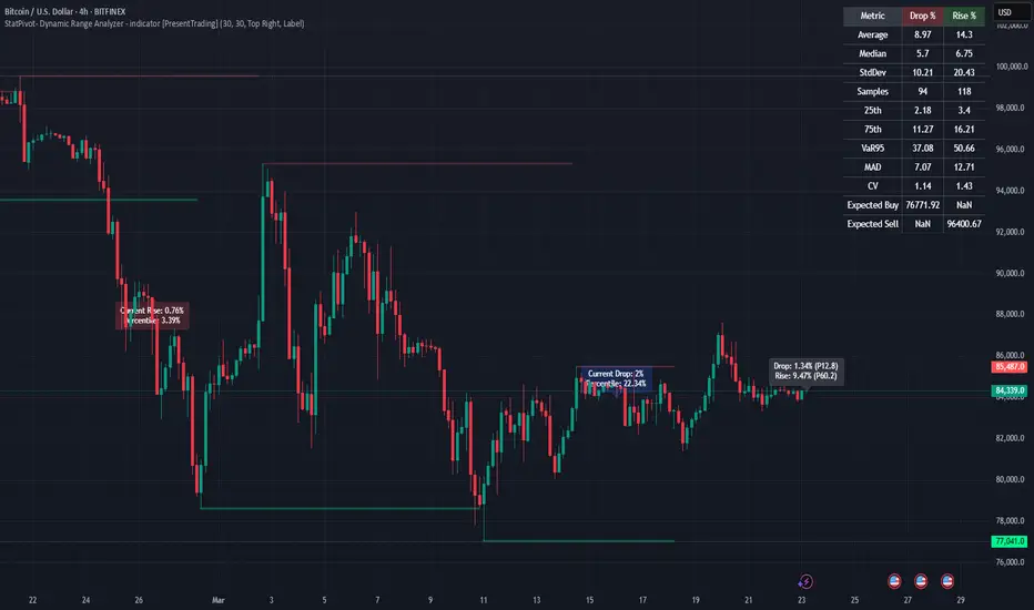
StatPivot- Dynamic Range Analyzer - indicator [PresentTrading]Hello everyone! In the following few open scripts, I would like to share various statistical tools that benefit trading. For this time, it is a powerful indicator called StatPivot- Dynamic Range Analyzer that brings a whole new dimension to your technical analysis toolkit.
This tool goes beyond traditional pivot point analysis by providing comprehensive statistical insights about price movements, helping you identify high-probability trading opportunities based on historical data patterns rather than subjective interpretations. Whether you're a day trader, swing trader, or position trader, StatPivot's real-time percentile rankings give you a statistical edge in understanding exactly where current price action stands within historical contexts.
Welcome to share your opinions! Looking forward to sharing the next tool soon!
█ Introduction and How it is Different
StatPivot is an advanced technical analysis tool that revolutionizes retracement analysis. Unlike traditional pivot indicators that only show static support/resistance levels, StatPivot delivers dynamic statistical insights based on historical pivot patterns.
Its key innovation is real-time percentile calculation - while conventional tools require new pivot formations before updating (often too late for trading decisions), StatPivot continuously analyzes where current price stands within historical retracement distributions.
Furthermore, StatPivot provides comprehensive statistical metrics including mean, median, standard deviation, and percentile distributions of price movements, giving traders a probabilistic edge by revealing which price levels represent statistically significant zones for potential reversals or continuations. By transforming raw price data into statistical insights, StatPivot helps traders move beyond subjective price analysis to evidence-based decision making.
█ Strategy, How it Works: Detailed Explanation
🔶 Pivot Point Detection and Analysis
The core of StatPivot's functionality begins with identifying significant pivot points in the price structure. Using the parameters left and right, the indicator locates pivot highs and lows by examining a specified number of bars to the left and right of each potential pivot point:
Copyp_low = ta.pivotlow(low, left, right)
p_high = ta.pivothigh(high, left, right)
For a point to qualify as a pivot low, it must have left higher lows to its left and right higher lows to its right. Similarly, a pivot high must have left lower highs to its left and right lower highs to its right. This approach ensures that only significant turning points are recognized.
🔶 Percentage Change Calculation
Once pivot points are identified, StatPivot calculates the percentage changes between consecutive pivot points:
For drops (when a pivot low is lower than the previous pivot low):
CopydropPercent = (previous_pivot_low - current_pivot_low) / previous_pivot_low * 100
For rises (when a pivot high is higher than the previous pivot high):
CopyrisePercent = (current_pivot_high - previous_pivot_high) / previous_pivot_high * 100
These calculations quantify the magnitude of each market swing, allowing for statistical analysis of historical price movements.
🔶 Statistical Distribution Analysis
StatPivot computes comprehensive statistics on the historical distribution of drops and rises:
Average (Mean): The arithmetic mean of all recorded percentage changes
CopyavgDrop = array.avg(dropValues)
Median: The middle value when all percentage changes are arranged in order
CopymedianDrop = array.median(dropValues)
Standard Deviation: Measures the dispersion of percentage changes from the average
CopystdDevDrop = array.stdev(dropValues)
Percentiles (25th, 75th): Values below which 25% and 75% of observations fall
Copyq1 = array.get(sorted, math.floor(cnt * 0.25))
q3 = array.get(sorted, math.floor(cnt * 0.75))
VaR95: The maximum expected percentage drop with 95% confidence
Copyvar95D = array.get(sortedD, math.floor(nD * 0.95))
Coefficient of Variation (CV): Measures relative variability
CopycvD = stdDevDrop / avgDrop
These statistics provide a comprehensive view of market behavior, enabling traders to understand the typical ranges and extreme moves.
🔶 Real-time Percentile Ranking
StatPivot's most innovative feature is its real-time percentile calculation. For each current price, it calculates:
The percentage drop from the latest pivot high:
CopycurrentDropPct = (latestPivotHigh - close) / latestPivotHigh * 100
The percentage rise from the latest pivot low:
CopycurrentRisePct = (close - latestPivotLow) / latestPivotLow * 100
The percentile ranks of these values within the historical distribution:
CopyrealtimeDropRank = (count of historical drops <= currentDropPct) / total drops * 100
This calculation reveals exactly where the current price movement stands in relation to all historical movements, providing crucial context for decision-making.
🔶 Cluster Analysis
To identify the most common retracement zones, StatPivot performs a cluster analysis by dividing the range of historical drops into five equal intervals:
CopyrangeSize = maxVal - minVal
For each interval boundary:
Copyboundaries = minVal + rangeSize * i / 5
By counting the number of observations in each interval, the indicator identifies the most frequently occurring retracement zones, which often serve as significant support or resistance areas.
🔶 Expected Price Targets
Using the statistical data, StatPivot calculates expected price targets:
CopytargetBuyPrice = close * (1 - avgDrop / 100)
targetSellPrice = close * (1 + avgRise / 100)
These targets represent statistically probable price levels for potential entries and exits based on the average historical behavior of the market.
█ Trade Direction
StatPivot functions as an analytical tool rather than a direct trading signal generator, providing statistical insights that can be applied to various trading strategies. However, the data it generates can be interpreted for different trade directions:
For Long Trades:
Entry considerations: Look for price drops that reach the 70-80th percentile range in the historical distribution, suggesting a statistically significant retracement
Target setting: Use the Expected Sell price or consider the average rise percentage as a reasonable target
Risk management: Set stop losses below recent pivot lows or at a distance related to the statistical volatility (standard deviation)
For Short Trades:
Entry considerations: Look for price rises that reach the 70-80th percentile range, indicating an unusual extension
Target setting: Use the Expected Buy price or average drop percentage as a target
Risk management: Set stop losses above recent pivot highs or based on statistical measures of volatility
For Range Trading:
Use the most common drop and rise clusters to identify probable reversal zones
Trade bounces between these statistically significant levels
For Trend Following:
Confirm trend strength by analyzing consecutive higher pivot lows (uptrend) or lower pivot highs (downtrend)
Use lower percentile retracements (20-30th percentile) as entry opportunities in established trends
█ Usage
StatPivot offers multiple ways to integrate its statistical insights into your trading workflow:
Statistical Table Analysis: Review the comprehensive statistics displayed in the data table to understand the market's behavior. Pay particular attention to:
Average drop and rise percentages to set reasonable expectations
Standard deviation to gauge volatility
VaR95 for risk assessment
Real-time Percentile Monitoring: Watch the real-time percentile display to see where the current price movement stands within the historical distribution. This can help identify:
Extreme movements (90th+ percentile) that might indicate reversal opportunities
Typical retracements (40-60th percentile) that might continue further
Shallow pullbacks (10-30th percentile) that might represent continuation opportunities in trends
Support and Resistance Identification: Utilize the plotted pivot points as key support and resistance levels, especially when they align with statistically significant percentile ranges.
Target Price Setting: Use the expected buy and sell prices calculated from historical averages as initial targets for your trades.
Risk Management: Apply the statistical measurements like standard deviation and VaR95 to set appropriate stop loss levels that account for the market's historical volatility.
Pattern Recognition: Over time, learn to recognize when certain percentile levels consistently lead to reversals or continuations in your specific market, and develop personalized strategies based on these observations.
█ Default Settings
The default settings of StatPivot have been carefully calibrated to provide reliable statistical analysis across a variety of markets and timeframes, but understanding their effects allows for optimal customization:
Left Bars (30) and Right Bars (30): These parameters determine how pivot points are identified. With both set to 30 by default:
A pivot low must be the lowest point among 30 bars to its left and 30 bars to its right
A pivot high must be the highest point among 30 bars to its left and 30 bars to its right
Effect on performance: Larger values create fewer but more significant pivot points, reducing noise but potentially missing important market structures. Smaller values generate more pivot points, capturing more nuanced movements but potentially including noise.
Table Position (Top Right): Determines where the statistical data table appears on the chart.
Effect on performance: No impact on analytical performance, purely a visual preference.
Show Distribution Histogram (False): Controls whether the distribution histogram of drop percentages is displayed.
Effect on performance: Enabling this provides visual insight into the distribution of retracements but can clutter the chart.
Show Real-time Percentile (True): Toggles the display of real-time percentile rankings.
Effect on performance: A critical setting that enables the dynamic analysis of current price movements. Disabling this removes one of the key advantages of the indicator.
Real-time Percentile Display Mode (Label): Chooses between label display or indicator line for percentile rankings.
Effect on performance: Labels provide precise information at the current price point, while indicator lines show the evolution of percentile rankings over time.
Advanced Considerations for Settings Optimization:
Timeframe Adjustment: Higher timeframes generally benefit from larger Left/Right values to identify truly significant pivots, while lower timeframes may require smaller values to capture shorter-term swings.
Volatility-Based Tuning: In highly volatile markets, consider increasing the Left/Right values to filter out noise. In less volatile conditions, lower values can help identify more potential entry and exit points.
Market-Specific Optimization: Different markets (forex, stocks, commodities) display different retracement patterns. Monitor the statistics table to see if your market typically shows larger or smaller retracements than the current settings are optimized for.
Trading Style Alignment: Adjust the settings to match your trading timeframe. Day traders might prefer settings that identify shorter-term pivots (smaller Left/Right values), while swing traders benefit from more significant pivots (larger Left/Right values).
By understanding how these settings affect the analysis and customizing them to your specific market and trading style, you can maximize the effectiveness of StatPivot as a powerful statistical tool for identifying high-probability trading opportunities.
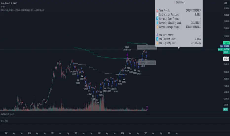
DCA Simulation for CryptoCommunity v1.1Overview
This script provides a detailed simulation of a Dollar-Cost Averaging (DCA) strategy tailored for crypto traders. It allows users to visualize how their DCA strategy would perform historically under specific parameters. The script is designed to help traders understand the mechanics of DCA and how it influences average price movement, budget utilization, and trade outcomes.
Key Features:
Combines Interval and Safety Order DCA:
Interval DCA: Regular purchases based on predefined time intervals.
Safety Order DCA: Additional buys triggered by percentage price drops.
Interactive Visualization:
Displays buy levels, average price, and profit-taking points on the chart.
Allows traders to assess how their strategy adapts to price movements.
Comprehensive Dashboard:
Tracks money spent, contracts acquired, and budget utilization.
Shows maximum amounts used if profit-taking is active.
Dynamic Safety Orders:
Resets safety orders when a new higher high is established.
Customizable Parameters:
Adjustable buy frequency, safety order settings, and profit-taking levels.
Suitable for traders with varying budgets and risk tolerances.
Default Strategy Settings:
Account Size: Default account size is set to $10,000 to represent a realistic budget for the average trader.
Commission & Slippage: Includes realistic trading fees and slippage assumptions to ensure accurate backtesting results.
Risk Management: Defaults to risking no more than 5% of the account balance per trade.
Sample Size: Optimized to generate a minimum of 100 trades for meaningful statistical analysis. Users can adjust parameters to fit longer timeframes or different datasets.
Usage Instructions:
Configure Your Strategy: Set the base order, safety order size, and buy frequency based on your preferred DCA approach.
Analyze Historical Performance: Use the chart and dashboard to understand how the strategy performs under different market conditions.
Optimize Parameters: Adjust settings to align with your risk tolerance and trading objectives.
Important Notes:
This script is for educational and simulation purposes. It is not intended to provide financial advice or guarantee profitability.
If the strategy's default settings do not meet your needs, feel free to adjust them while keeping risk management in mind.
TradingView limits the number of open trades to 999, so reduce the buy frequency if necessary to fit longer timeframes.
MathHelpersLibrary "MathHelpers"
Overview
A collection of helper functions for designing indicators and strategies.
calculateATR(length, log)
Calculates the Average True Range (ATR) or Log ATR based on the 'log' parameter. Sans Wilder's Smoothing
Parameters:
length (simple int)
log (simple bool)
Returns: float The calculated ATR value. Returns Log ATR if `log` is true, otherwise returns standard ATR.
CDF(z)
Computes the Cumulative Distribution Function (CDF) for a given value 'z', mimicking the CDF function in "Statistically Sound Indicators" by Timothy Masters.
Parameters:
z (simple float)
Returns: float The CDF value corresponding to the input `z`, ranging between 0 and 1.
logReturns(lookback)
Calculates the logarithmic returns over a specified lookback period.
Parameters:
lookback (simple int)
Returns: float The calculated logarithmic return. Returns `na` if insufficient data is available.
Volume StatsDescription:
Volume Stats displays volume data and statistics for every day of the year, and is designed to work on "1D" timeframe. The data is displayed in a table with columns being months of the year, and rows being days of each month. By default, latest data is displayed, but you have an option to switch to data of the previous year as well.
The statistics displayed for each day is:
- volume
- % of total yearly volume
- % of total monthly volume
The statistics displayed for each column (month) is:
- monthly volume
- % of total yearly volume
- sentiment (was there more bullish or bearish volume?)
- min volume (on which day of the month was the min volume)
- max volume (on which day of the month was the max volume)
The cells change their colors depending on whether the volume is bullish or bearish, and what % of total volume the current cell has (either yearly or monthly). The header cells also change their color (based either on sentiment or what % of yearly volume the current month has).
This is the first (and free) version of the indicator, and I'm planning to create a "PRO" version of this indicator in future.
Parameters:
- Timezone
- Cell data -> which data to display in the cells (no data, volume or percentage)
- Highlight min and max volume -> if checked, cells with min and max volume (either monthly or yearly) will be highlighted with a dot or letter (depending on the "Cell data" input)
- Cell stats mode -> which data to use for color and % calculation (All data = yearly, Column = monthly)
- Display data from previous year -> if checked, the data from previous year will be used
- Header color is calculated from -> either sentiment or % of the yearly volume
- Reverse theme -> the table colors are automatically changed based on the "Dark mode" of Tradingview, this checkbox reverses the logic (so that darker colors will be used when "Dark mode" is off, and lighter colors when it's on)
- Hide logo -> hides the cat logo (PLEASE DO NOT HIDE THE CAT)
Conclusion:
Let me know what you think of the indicator. As I said, I'm planning to make a PRO version with more features, for which I already have some ideas, but if you have any suggestions, please let me know.
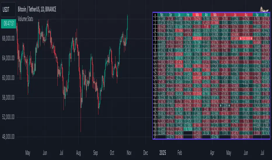
analytics_tablesLibrary "analytics_tables"
📝 Description
This library provides the implementation of several performance-related statistics and metrics, presented in the form of tables.
The metrics shown in the afforementioned tables where developed during the past years of my in-depth analalysis of various strategies in an atempt to reason about the performance of each strategy.
The visualization and some statistics where inspired by the existing implementations of the "Seasonality" script, and the performance matrix implementations of @QuantNomad and @ZenAndTheArtOfTrading scripts.
While this library is meant to be used by my strategy framework "Template Trailing Strategy (Backtester)" script, I wrapped it in a library hoping this can be usefull for other community strategy scripts that will be released in the future.
🤔 How to Guide
To use the functionality this library provides in your script you have to import it first!
Copy the import statement of the latest release by pressing the copy button below and then paste it into your script. Give a short name to this library so you can refer to it later on. The import statement should look like this:
import jason5480/analytics_tables/1 as ant
There are three types of tables provided by this library in the initial release. The stats table the metrics table and the seasonality table.
Each one shows different kinds of performance statistics.
The table UDT shall be initialized once using the `init()` method.
They can be updated using the `update()` method where the updated data UDT object shall be passed.
The data UDT can also initialized and get updated on demend depending on the use case
A code example for the StatsTable is the following:
var ant.StatsData statsData = ant.StatsData.new()
statsData.update(SideStats.new(), SideStats.new(), 0)
if (barstate.islastconfirmedhistory or (barstate.isrealtime and barstate.isconfirmed))
var statsTable = ant.StatsTable.new().init(ant.getTablePos('TOP', 'RIGHT'))
statsTable.update(statsData)
A code example for the MetricsTable is the following:
var ant.StatsData statsData = ant.StatsData.new()
statsData.update(ant.SideStats.new(), ant.SideStats.new(), 0)
if (barstate.islastconfirmedhistory or (barstate.isrealtime and barstate.isconfirmed))
var metricsTable = ant.MetricsTable.new().init(ant.getTablePos('BOTTOM', 'RIGHT'))
metricsTable.update(statsData, 10)
A code example for the SeasonalityTable is the following:
var ant.SeasonalData seasonalData = ant.SeasonalData.new().init(Seasonality.monthOfYear)
seasonalData.update()
if (barstate.islastconfirmedhistory or (barstate.isrealtime and barstate.isconfirmed))
var seasonalTable = ant.SeasonalTable.new().init(seasonalData, ant.getTablePos('BOTTOM', 'LEFT'))
seasonalTable.update(seasonalData)
🏋️♂️ Please refer to the "EXAMPLE" regions of the script for more advanced and up to date code examples!
Special thanks to @Mrcrbw for the proposal to develop this library and @DCNeu for the constructive feedback 🏆.
getTablePos(ypos, xpos)
Get table position compatible string
Parameters:
ypos (simple string) : The position on y axise
xpos (simple string) : The position on x axise
Returns: The position to be passed to the table
method init(this, pos, height, width, positiveTxtColor, negativeTxtColor, neutralTxtColor, positiveBgColor, negativeBgColor, neutralBgColor)
Initialize the stats table object with the given colors in the given position
Namespace types: StatsTable
Parameters:
this (StatsTable) : The stats table object
pos (simple string) : The table position string
height (simple float) : The height of the table as a percentage of the charts height. By default, 0 auto-adjusts the height based on the text inside the cells
width (simple float) : The width of the table as a percentage of the charts height. By default, 0 auto-adjusts the width based on the text inside the cells
positiveTxtColor (simple color) : The text color when positive
negativeTxtColor (simple color) : The text color when negative
neutralTxtColor (simple color) : The text color when neutral
positiveBgColor (simple color) : The background color with transparency when positive
negativeBgColor (simple color) : The background color with transparency when negative
neutralBgColor (simple color) : The background color with transparency when neutral
method init(this, pos, height, width, neutralBgColor)
Initialize the metrics table object with the given colors in the given position
Namespace types: MetricsTable
Parameters:
this (MetricsTable) : The metrics table object
pos (simple string) : The table position string
height (simple float) : The height of the table as a percentage of the charts height. By default, 0 auto-adjusts the height based on the text inside the cells
width (simple float) : The width of the table as a percentage of the charts width. By default, 0 auto-adjusts the width based on the text inside the cells
neutralBgColor (simple color) : The background color with transparency when neutral
method init(this, seas)
Initialize the seasonal data
Namespace types: SeasonalData
Parameters:
this (SeasonalData) : The seasonal data object
seas (simple Seasonality) : The seasonality of the matrix data
method init(this, data, pos, maxNumOfYears, height, width, extended, neutralTxtColor, neutralBgColor)
Initialize the seasonal table object with the given colors in the given position
Namespace types: SeasonalTable
Parameters:
this (SeasonalTable) : The seasonal table object
data (SeasonalData) : The seasonality data of the table
pos (simple string) : The table position string
maxNumOfYears (simple int) : The maximum number of years that fit into the table
height (simple float) : The height of the table as a percentage of the charts height. By default, 0 auto-adjusts the height based on the text inside the cells
width (simple float) : The width of the table as a percentage of the charts width. By default, 0 auto-adjusts the width based on the text inside the cells
extended (simple bool) : The seasonal table with extended columns for performance
neutralTxtColor (simple color) : The text color when neutral
neutralBgColor (simple color) : The background color with transparency when neutral
method update(this, wins, losses, numOfInconclusiveExits)
Update the strategy info data of the strategy
Namespace types: StatsData
Parameters:
this (StatsData) : The strategy statistics object
wins (SideStats)
losses (SideStats)
numOfInconclusiveExits (int) : The number of inconclusive trades
method update(this, stats, positiveTxtColor, negativeTxtColor, negativeBgColor, neutralBgColor)
Update the stats table object with the given data
Namespace types: StatsTable
Parameters:
this (StatsTable) : The stats table object
stats (StatsData) : The stats data to update the table
positiveTxtColor (simple color) : The text color when positive
negativeTxtColor (simple color) : The text color when negative
negativeBgColor (simple color) : The background color with transparency when negative
neutralBgColor (simple color) : The background color with transparency when neutral
method update(this, stats, buyAndHoldPerc, positiveTxtColor, negativeTxtColor, positiveBgColor, negativeBgColor)
Update the metrics table object with the given data
Namespace types: MetricsTable
Parameters:
this (MetricsTable) : The metrics table object
stats (StatsData) : The stats data to update the table
buyAndHoldPerc (float) : The buy and hold percetage
positiveTxtColor (simple color) : The text color when positive
negativeTxtColor (simple color) : The text color when negative
positiveBgColor (simple color) : The background color with transparency when positive
negativeBgColor (simple color) : The background color with transparency when negative
method update(this)
Update the seasonal data based on the season and eon timeframe
Namespace types: SeasonalData
Parameters:
this (SeasonalData) : The seasonal data object
method update(this, data, positiveTxtColor, negativeTxtColor, neutralTxtColor, positiveBgColor, negativeBgColor, neutralBgColor, timeBgColor)
Update the seasonal table object with the given data
Namespace types: SeasonalTable
Parameters:
this (SeasonalTable) : The seasonal table object
data (SeasonalData) : The seasonal cell data to update the table
positiveTxtColor (simple color) : The text color when positive
negativeTxtColor (simple color) : The text color when negative
neutralTxtColor (simple color) : The text color when neutral
positiveBgColor (simple color) : The background color with transparency when positive
negativeBgColor (simple color) : The background color with transparency when negative
neutralBgColor (simple color) : The background color with transparency when neutral
timeBgColor (simple color) : The background color of the time gradient
SideStats
Object that represents the strategy statistics data of one side win or lose
Fields:
numOf (series int)
sumFreeProfit (series float)
freeProfitStDev (series float)
sumProfit (series float)
profitStDev (series float)
sumGain (series float)
gainStDev (series float)
avgQuantityPerc (series float)
avgCapitalRiskPerc (series float)
avgTPExecutedCount (series float)
avgRiskRewardRatio (series float)
maxStreak (series int)
StatsTable
Object that represents the stats table
Fields:
table (series table) : The actual table
rows (series int) : The number of rows of the table
columns (series int) : The number of columns of the table
StatsData
Object that represents the statistics data of the strategy
Fields:
wins (SideStats)
losses (SideStats)
numOfInconclusiveExits (series int)
avgFreeProfitStr (series string)
freeProfitStDevStr (series string)
lossFreeProfitStDevStr (series string)
avgProfitStr (series string)
profitStDevStr (series string)
lossProfitStDevStr (series string)
avgQuantityStr (series string)
MetricsTable
Object that represents the metrics table
Fields:
table (series table) : The actual table
rows (series int) : The number of rows of the table
columns (series int) : The number of columns of the table
SeasonalData
Object that represents the seasonal table dynamic data
Fields:
seasonality (series Seasonality)
eonToMatrixRow (map)
numOfEons (series int)
mostRecentMatrixRow (series int)
balances (matrix)
returnPercs (matrix)
maxDDs (matrix)
eonReturnPercs (array)
eonCAGRs (array)
eonMaxDDs (array)
SeasonalTable
Object that represents the seasonal table
Fields:
table (series table) : The actual table
headRows (series int) : The number of head rows of the table
headColumns (series int) : The number of head columns of the table
eonRows (series int) : The number of eon rows of the table
seasonColumns (series int) : The number of season columns of the table
statsRows (series int)
statsColumns (series int) : The number of stats columns of the table
rows (series int) : The number of rows of the table
columns (series int) : The number of columns of the table
extended (series bool) : Whether the table has additional performance statistics

Portfolio Index Generator [By MUQWISHI]▋ INTRODUCTION:
The “Portfolio Index Generator” simplifies the process of building a custom portfolio management index, allowing investors to input a list of preferred holdings from global securities and customize the initial investment weight of each security. Furthermore, it includes an option for rebalancing by adjusting the weights of assets to maintain a desired level of asset allocation. The tool serves as a comprehensive approach for tracking portfolio performance, conducting research, and analyzing specific aspects of portfolio investment. The output includes an index value, a table of holdings, and chart plotting, providing a deeper understanding of the portfolio's historical movement.
_______________________
▋ OVERVIEW:
The image can be taken as an example of building a custom portfolio index. I created this index and named it “My Portfolio Performance”, which comprises several global companies and crypto assets.
_______________________
▋ OUTPUTS:
The output can be divided into 4 sections:
1. Portfolio Index Title (Name & Value).
2. Portfolio Specifications.
3. Portfolio Holdings.
4. Portfolio Index Chart.
1. Portfolio Index Title, displays the index name at the top, and at the bottom, it shows the index value, along with the chart timeframe, e.g., daily change in points and percentage.
2. Portfolio Specifications, displays the essential information on portfolio performance, including the investment date range, initial capital, returns, assets, and equity.
3. Portfolio Holdings, a list of the holding securities inside a table that contains the ticker, average entry price, last price, return percentage of the portfolio's initial capital, and customized weighted percentage of the portfolio. Additionally, a tooltip appears when the user passes the cursor over a ticker's cell, showing brief information about the company, such as the company's name, exchange market, country, sector, and industry.
4. Index Chart, display a plot of the historical movement of the index in the form of a bar, candle, or line chart.
_______________________
▋ INDICATOR SETTINGS:
Section(1): Style Settings
(1) Naming the index.
(2) Table location on the chart and cell size.
(3) Sorting Holdings Table. By securities’ {Return(%) Portfolio, Weight(%) Portfolio, or Ticker Alphabetical} order.
(4) Choose the type of index: {Equity or Return (%)}, and the plot type for the index: {Candle, Bar, or Line}.
(5) Positive/Negative colors.
(6) Table Colors (Title, Cell, and Text).
(7) To show/hide any indicator’s components.
Section(2): Performance Settings
(1) Calculation window period: from DateTime to DateTime.
(2) Initial Capital and specifying currency.
(3) Option to enable portfolio rebalancing in {Monthly, Quarterly, or Yearly} intervals.
Section(3): Portfolio Holdings
(1) Enable and count security in the investment portfolio.
(2) Initial weight of security. For example, if the initial capital is $100,000 and the weight of XYZ stock is 4%, the initial value of the shares would be $4,000.
(3) Select and add up to 30 symbols that interested in.
Please let me know if you have any questions.

Volatility and Volume by Hour EXT(Extended republication, use this instead of the old one)
The goal of this indicator is to show a “characteristic” of the instrument, regarding the price change and trading volume. You can see how the instrument “behaved” throughout the day in the lookback period. I've found this useful for timing in day trading.
The indicator creates a table on the chart to display various statistics for each hour of the day.
Important: ONLY SHOWS THE TABLE IF THE CHART’S TIMEFRAME IS 1H!
Explanation of the columns:
1. Volatility Percentage (Volat): This column shows the volatility of the price as a percentage. For example, a value of "15%" means the price movement was 15% of the total daily price movement within the hour.
2. Hourly Point Change (PointCh): This column shows the change in price points for each hour in the lookback period. For example, a value of "5" means the price has increased by 5 points in the hour, while "-3" means it has decreased by 3 points.
3. Hourly Point Change Percentage (PrCh% (LeverageX)): This column shows the percentage change in price points for each hour, adjusted with leverage multiplier. Displayed green (+) or red (-) accordingly. For example, a value of "10%" with a leverage of 2X means the price has effectively changed by 5% due to the leverage.
4. Trading Volume Percentage (TrVol): This column shows the percentage of the daily total volume that was traded in a specific hour. For example, a value of "10%" would mean that 10% of the day's total trading volume occurred in that hour.
5. Added New! - Relevancy Check: The indicator checks the last 24 candle. If the direction of the price movement was the same in the last 24 hour as the statistical direction in that hour, the background of the relevant hour in the second column goes green.
For example: if today at 9 o'clock the price went lower, so as at 9 o'clock in the loopback period, the instrument "behaves" according to statistics . So the statistics is probably more relevant for today. The more green background row the more relevancy.
Settings:
1. Lookback period: The lookback period is the number of previous bars from which data is taken to perform calculations. In this script, it's used in a loop that iterates over a certain number of past bars to calculate the statistics. TIP: Select a period the contains a trend in one direction, because an upward and a downward trend compensate the price movement in opposite directions.
2. Timezone: This is a string input that represents the user's timezone. The default value is "UTC+2". Adjust it to your timezone in order to view the hours properly.
3. Leverage: The default value is 10(!). This input is used to adjust the hourly point change percentage. For FOREX traders (for example) the statistics can show the leveraged percentage of price change. Set that according the leverage you trade the instrument with.
Use at your own risk, provided “as is” basis!
Hope you find it useful! Cheers!
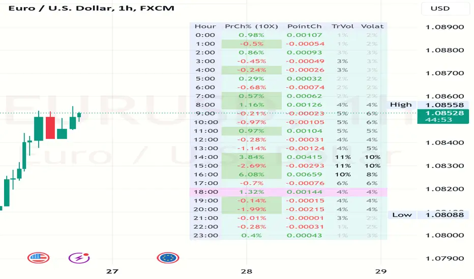
trend_switch
█ Description
Asset price data was time series data, commonly consisting of trends, seasonality, and noise. Many applicable indicators help traders to determine between trend or momentum to make a better trading decision based on their preferences. In some cases, there is little to no clear market direction, and price range. It feels much more appropriate to use a shorter trend identifier, until clearly defined market trend. The indicator/strategy developed with the notion aims to automatically switch between shorter and longer trend following indicator. There were many methods that can be applied and switched between, however in this indicator/strategy will be limited to the use of predictive moving average and MESA adaptive moving average (Ehlers), by first determining if there is a strong trend identified by calculating the slope, if slope value is between upper and lower threshold assumed there is not much price direction.
█ Formula
// predictive moving average
predict = (2*wma1-wma2)
trigger = (4*predict+3*predict +2*predict *predict)
// MESA adaptive moving average
mama = alpha*src+(1-alpha)*mama
fama = .5*alpha*mama+(1-.5-alpha)*fama
█ Feature
The indicator will have a specified default parameter of:
source = ohlc4
lookback period = 10
threshold = 10
fast limit = 0.5
slow limit = 0.05
Strategy type can be switched between Long/Short only and Long-Short strategy
Strategy backtest period
█ How it works
If slope between the upper (red) and lower (green) threshold line, assume there is little to no clear market direction, thus signal predictive moving average indicator
If slope is above the upper (red) or below the lower (green) threshold line, assume there is a clear trend forming, the signal generated from the MESA adaptive moving average indicator
█ Example 1 - Slope fall between the Threshold - activate shorter trend
█ Example 2 - Slope fall above/below Threshold - activate longer trend

Inflation CorrelationHeyo fellas,
In today’s dynamic economic landscape, understanding the relationship of market prices to other economical factors like inflation rate is crucial. The Inflation Correlation Indicator is designed to provide traders with a clear visualization of this relationship. By correlating average inflation rates from selected countries with market closing prices, this indicator offers a unique perspective on potential market movements influenced by inflationary trends.
Features:
Country Selection: Choose from the European Union (EU), Germany (DE), or the United States (US) to tailor the correlation analysis to your specific market interest.
Correlation Length Customization: Adjust the correlation length to refine the sensitivity of the indicator to recent inflation data.
Visual Clarity: The correlation histogram changes color based on the direction of the correlation, providing an intuitive understanding of the inflation correlation.
Whether you’re a fundamental analyst seeking to incorporate macroeconomic indicators into your strategy or a trader looking for an edge in inflation-sensitive markets, the Inflation Correlation Indicator is an indispensable tool in your TradingView arsenal.
Thanks for checking this out!
Best regards,
simwai
Statistics • Chi Square • P-value • SignificanceThe Statistics • Chi Square • P-value • Significance publication aims to provide a tool for combining different conditions and checking whether the outcome is significant using the Chi-Square Test and P-value.
🔶 USAGE
The basic principle is to compare two or more groups and check the results of a query test, such as asking men and women whether they want to see a romantic or non-romantic movie.
–––––––––––––––––––––––––––––––––––––––––––––
| | ROMANTIC | NON-ROMANTIC | ⬅︎ MOVIE |
–––––––––––––––––––––––––––––––––––––––––––––
| MEN | 2 | 8 | 10 |
–––––––––––––––––––––––––––––––––––––––––––––
| WOMEN | 7 | 3 | 10 |
–––––––––––––––––––––––––––––––––––––––––––––
|⬆︎ SEX | 10 | 10 | 20 |
–––––––––––––––––––––––––––––––––––––––––––––
We calculate the Chi-Square Formula, which is:
Χ² = Σ ( (Observed Value − Expected Value)² / Expected Value )
In this publication, this is:
chiSquare = 0.
for i = 0 to rows -1
for j = 0 to colums -1
observedValue = aBin.get(i).aFloat.get(j)
expectedValue = math.max(1e-12, aBin.get(i).aFloat.get(colums) * aBin.get(rows).aFloat.get(j) / sumT) //Division by 0 protection
chiSquare += math.pow(observedValue - expectedValue, 2) / expectedValue
Together with the 'Degree of Freedom', which is (rows − 1) × (columns − 1) , the P-value can be calculated.
In this case it is P-value: 0.02462
A P-value lower than 0.05 is considered to be significant. Statistically, women tend to choose a romantic movie more, while men prefer a non-romantic one.
Users have the option to choose a P-value, calculated from a standard table or through a math.ucla.edu - Javascript-based function (see references below).
Note that the population (10 men + 10 women = 20) is small, something to consider.
Either way, this principle is applied in the script, where conditions can be chosen like rsi, close, high, ...
🔹 CONDITION
Conditions are added to the left column ('CONDITION')
For example, previous rsi values (rsi ) between 0-100, divided in separate groups
🔹 CLOSE
Then, the movement of the last close is evaluated
UP when close is higher then previous close (close )
DOWN when close is lower then previous close
EQUAL when close is equal then previous close
It is also possible to use only 2 columns by adding EQUAL to UP or DOWN
UP
DOWN/EQUAL
or
UP/EQUAL
DOWN
In other words, when previous rsi value was between 80 and 90, this resulted in:
19 times a current close higher than previous close
14 times a current close lower than previous close
0 times a current close equal than previous close
However, the P-value tells us it is not statistical significant.
NOTE: Always keep in mind that past behaviour gives no certainty about future behaviour.
A vertical line is drawn at the beginning of the chosen population (max 4990)
Here, the results seem significant.
🔹 GROUPS
It is important to ensure that the groups are formed correctly. All possibilities should be present, and conditions should only be part of 1 group.
In the example above, the two top situations are acceptable; close against close can only be higher, lower or equal.
The two examples at the bottom, however, are very poorly constructed.
Several conditions can be placed in more than 1 group, and some conditions are not integrated into a group. Even if the results are significant, they are useless because of the group formation.
A population count is added as an aid to spot errors in group formation.
In this example, there is a discrepancy between the population and total count due to the absence of a condition.
The results when rsi was between 5-25 are not included, resulting in unreliable results.
🔹 PRACTICAL EXAMPLES
In this example, we have specific groups where the condition only applies to that group.
For example, the condition rsi > 55 and rsi <= 65 isn't true in another group.
Also, every possible rsi value (0 - 100) is present in 1 of the groups.
rsi > 15 and rsi <= 25 28 times UP, 19 times DOWN and 2 times EQUAL. P-value: 0.01171
When looking in detail and examining the area 15-25 RSI, we see this:
The population is now not representative (only checking for RSI between 15-25; all other RSI values are not included), so we can ignore the P-value in this case. It is merely to check in detail. In this case, the RSI values 23 and 24 seem promising.
NOTE: We should check what the close price did without any condition.
If, for example, the close price had risen 100 times out of 100, this would make things very relative.
In this case (at least two conditions need to be present), we set 1 condition at 'always true' and another at 'always false' so we'll get only the close values without any condition:
Changing the population or the conditions will change the P-value.
In the following example, the outcome is evaluated when:
close value from 1 bar back is higher than the close value from 2 bars back
close value from 1 bar back is lower/equal than the close value from 2 bars back
Or:
close value from 1 bar back is higher than the close value from 2 bars back
close value from 1 bar back is equal than the close value from 2 bars back
close value from 1 bar back is lower than the close value from 2 bars back
In both examples, all possibilities of close against close are included in the calculations. close can only by higher, equal or lower than close
Both examples have the results without a condition included (5 = 5 and 5 < 5) so one can compare the direction of current close.
🔶 NOTES
• Always keep in mind that:
Past behaviour gives no certainty about future behaviour.
Everything depends on time, cycles, events, fundamentals, technicals, ...
• This test only works for categorical data (data in categories), such as Gender {Men, Women} or color {Red, Yellow, Green, Blue} etc., but not numerical data such as height or weight. One might argue that such tests shouldn't use rsi, close, ... values.
• Consider what you're measuring
For example rsi of the current bar will always lead to a close higher than the previous close, since this is inherent to the rsi calculations.
• Be careful; often, there are na -values at the beginning of the series, which are not included in the calculations!
• Always keep in mind considering what the close price did without any condition
• The numbers must be large enough. Each entry must be five or more. In other words, it is vital to make the 'population' large enough.
• The code can be developed further, for example, by splitting UP, DOWN in close UP 1-2%, close UP 2-3%, close UP 3-4%, ...
• rsi can be supplemented with stochRSI, MFI, sma, ema, ...
🔶 SETTINGS
🔹 Population
• Choose the population size; in other words, how many bars you want to go back to. If fewer bars are available than set, this will be automatically adjusted.
🔹 Inputs
At least two conditions need to be chosen.
• Users can add up to 11 conditions, where each condition can contain two different conditions.
🔹 RSI
• Length
🔹 Levels
• Set the used levels as desired.
🔹 Levels
• P-value: P-value retrieved using a standard table method or a function.
• Used function, derived from Chi-Square Distribution Function; JavaScript
LogGamma(Z) =>
S = 1
+ 76.18009173 / Z
- 86.50532033 / (Z+1)
+ 24.01409822 / (Z+2)
- 1.231739516 / (Z+3)
+ 0.00120858003 / (Z+4)
- 0.00000536382 / (Z+5)
(Z-.5) * math.log(Z+4.5) - (Z+4.5) + math.log(S * 2.50662827465)
Gcf(float X, A) => // Good for X > A +1
A0=0., B0=1., A1=1., B1=X, AOLD=0., N=0
while (math.abs((A1-AOLD)/A1) > .00001)
AOLD := A1
N += 1
A0 := A1+(N-A)*A0
B0 := B1+(N-A)*B0
A1 := X*A0+N*A1
B1 := X*B0+N*B1
A0 := A0/B1
B0 := B0/B1
A1 := A1/B1
B1 := 1
Prob = math.exp(A * math.log(X) - X - LogGamma(A)) * A1
1 - Prob
Gser(X, A) => // Good for X < A +1
T9 = 1. / A
G = T9
I = 1
while (T9 > G* 0.00001)
T9 := T9 * X / (A + I)
G := G + T9
I += 1
G *= math.exp(A * math.log(X) - X - LogGamma(A))
Gammacdf(x, a) =>
GI = 0.
if (x<=0)
GI := 0
else if (x
Chisqcdf = Gammacdf(Z/2, DF/2)
Chisqcdf := math.round(Chisqcdf * 100000) / 100000
pValue = 1 - Chisqcdf
🔶 REFERENCES
mathsisfun.com, Chi-Square Test
Chi-Square Distribution Function
Wick %Heyo Fellas,
thanks for checking out my new indicator.
Introduction
Wick % is a simple indicator to compare wick size with body size (mode 1) and to compare wick size with candle size (mode 2).
Upper wicks are bullish when close is higher than open pricen.
Lower wicks are bearish when close is lower than open price.
Wick Theory
In general, big wick and small bodie on a bar means that bull and bears are fighting heavily.
A big wick below the body means the bulls are leading in that fight,
and a big wick above the body means the bears are leading in that fight.
Calculation Formula
Mode 1 – Percentual Increase Wick/Body:
upperWickPercentage = (upperWick / body) * 100 - 100
lowerWickPercentage = (lowerWick / body) * 100 - 100
Mode 2 – Percent Wick/Candlestick:
upperWickPercentage = (upperWick / (high - low)) * 100
lowerWickPercentage = (lowerWick / (high - low)) * 100
Usage
You can use it on every symbol and every timeframe.
The indicator repaints by default, but you can disable it in the settings.
When you disable repaint, it moves the label one bar to the right.
If you want to use the indicator for signals, you must disable repainting.
Best regards,
simwai
Likelihood of Winning - Probability Density FunctionIn developing the "Likelihood of Winning - Probability Density Function (PDF)" indicator, my aim was to offer traders a statistical tool to quantify the probability of reaching target prices. This indicator, grounded in risk assessment principles, enables users to analyze potential outcomes based on the normal distribution, providing insights into market dynamics.
The tool's flexibility allows for customization of the data series, lookback periods, and target settings for both long and short scenarios. It features a color-coded visualization to easily distinguish between probabilities of hitting specified targets, enhancing decision-making in trading strategies.
I'm excited to share this indicator with the trading community, hoping it will enhance data-driven decision-making and offer a deeper understanding of market risks and opportunities. My goal is to continuously improve this tool based on user feedback and market evolution, contributing to more informed trading practices.
This indicator leverages the "NormalDistributionFunctions" library, enabling easy integration into other indicators or strategies. Users can readily embed advanced statistical analysis into their trading tools, fostering innovation within the Pine Script community.