UtilityLibrary "Utility"
dema(src, length)
Parameters:
src (float)
length (simple int)
tema(src, length)
Parameters:
src (float)
length (simple int)
hma(src, length)
Parameters:
src (float)
length (int)
zlema(src, length)
Parameters:
src (float)
length (simple int)
stochRSI(src, lengthRSI, lengthStoch, smoothK, smoothD)
Parameters:
src (float)
lengthRSI (simple int)
lengthStoch (int)
smoothK (int)
smoothD (int)
slope(src, length)
Parameters:
src (float)
length (int)
Statistics

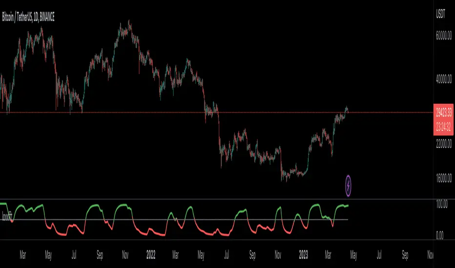
loxxfftLibrary "loxxfft"
This code is a library for performing Fast Fourier Transform (FFT) operations. FFT is an algorithm that can quickly compute the discrete Fourier transform (DFT) of a sequence. The library includes functions for performing FFTs on both real and complex data. It also includes functions for fast correlation and convolution, which are operations that can be performed efficiently using FFTs. Additionally, the library includes functions for fast sine and cosine transforms.
Reference:
www.alglib.net
fastfouriertransform(a, nn, inversefft)
Returns Fast Fourier Transform
Parameters:
a (float ) : float , An array of real and imaginary parts of the function values. The real part is stored at even indices, and the imaginary part is stored at odd indices.
nn (int) : int, The number of function values. It must be a power of two, but the algorithm does not validate this.
inversefft (bool) : bool, A boolean value that indicates the direction of the transformation. If True, it performs the inverse FFT; if False, it performs the direct FFT.
Returns: float , Modifies the input array a in-place, which means that the transformed data (the FFT result for direct transformation or the inverse FFT result for inverse transformation) will be stored in the same array a after the function execution. The transformed data will have real and imaginary parts interleaved, with the real parts at even indices and the imaginary parts at odd indices.
realfastfouriertransform(a, tnn, inversefft)
Returns Real Fast Fourier Transform
Parameters:
a (float ) : float , A float array containing the real-valued function samples.
tnn (int) : int, The number of function values (must be a power of 2, but the algorithm does not validate this condition).
inversefft (bool) : bool, A boolean flag that indicates the direction of the transformation (True for inverse, False for direct).
Returns: float , Modifies the input array a in-place, meaning that the transformed data (the FFT result for direct transformation or the inverse FFT result for inverse transformation) will be stored in the same array a after the function execution.
fastsinetransform(a, tnn, inversefst)
Returns Fast Discrete Sine Conversion
Parameters:
a (float ) : float , An array of real numbers representing the function values.
tnn (int) : int, Number of function values (must be a power of two, but the code doesn't validate this).
inversefst (bool) : bool, A boolean flag indicating the direction of the transformation. If True, it performs the inverse FST, and if False, it performs the direct FST.
Returns: float , The output is the transformed array 'a', which will contain the result of the transformation.
fastcosinetransform(a, tnn, inversefct)
Returns Fast Discrete Cosine Transform
Parameters:
a (float ) : float , This is a floating-point array representing the sequence of values (time-domain) that you want to transform. The function will perform the Fast Cosine Transform (FCT) or the inverse FCT on this input array, depending on the value of the inversefct parameter. The transformed result will also be stored in this same array, which means the function modifies the input array in-place.
tnn (int) : int, This is an integer value representing the number of data points in the input array a. It is used to determine the size of the input array and control the loops in the algorithm. Note that the size of the input array should be a power of 2 for the Fast Cosine Transform algorithm to work correctly.
inversefct (bool) : bool, This is a boolean value that controls whether the function performs the regular Fast Cosine Transform or the inverse FCT. If inversefct is set to true, the function will perform the inverse FCT, and if set to false, the regular FCT will be performed. The inverse FCT can be used to transform data back into its original form (time-domain) after the regular FCT has been applied.
Returns: float , The resulting transformed array is stored in the input array a. This means that the function modifies the input array in-place and does not return a new array.
fastconvolution(signal, signallen, response, negativelen, positivelen)
Convolution using FFT
Parameters:
signal (float ) : float , This is an array of real numbers representing the input signal that will be convolved with the response function. The elements are numbered from 0 to SignalLen-1.
signallen (int) : int, This is an integer representing the length of the input signal array. It specifies the number of elements in the signal array.
response (float ) : float , This is an array of real numbers representing the response function used for convolution. The response function consists of two parts: one corresponding to positive argument values and the other to negative argument values. Array elements with numbers from 0 to NegativeLen match the response values at points from -NegativeLen to 0, respectively. Array elements with numbers from NegativeLen+1 to NegativeLen+PositiveLen correspond to the response values in points from 1 to PositiveLen, respectively.
negativelen (int) : int, This is an integer representing the "negative length" of the response function. It indicates the number of elements in the response function array that correspond to negative argument values. Outside the range , the response function is considered zero.
positivelen (int) : int, This is an integer representing the "positive length" of the response function. It indicates the number of elements in the response function array that correspond to positive argument values. Similar to negativelen, outside the range , the response function is considered zero.
Returns: float , The resulting convolved values are stored back in the input signal array.
fastcorrelation(signal, signallen, pattern, patternlen)
Returns Correlation using FFT
Parameters:
signal (float ) : float ,This is an array of real numbers representing the signal to be correlated with the pattern. The elements are numbered from 0 to SignalLen-1.
signallen (int) : int, This is an integer representing the length of the input signal array.
pattern (float ) : float , This is an array of real numbers representing the pattern to be correlated with the signal. The elements are numbered from 0 to PatternLen-1.
patternlen (int) : int, This is an integer representing the length of the pattern array.
Returns: float , The signal array containing the correlation values at points from 0 to SignalLen-1.
tworealffts(a1, a2, a, b, tn)
Returns Fast Fourier Transform of Two Real Functions
Parameters:
a1 (float ) : float , An array of real numbers, representing the values of the first function.
a2 (float ) : float , An array of real numbers, representing the values of the second function.
a (float ) : float , An output array to store the Fourier transform of the first function.
b (float ) : float , An output array to store the Fourier transform of the second function.
tn (int) : float , An integer representing the number of function values. It must be a power of two, but the algorithm doesn't validate this condition.
Returns: float , The a and b arrays will contain the Fourier transform of the first and second functions, respectively. Note that the function overwrites the input arrays a and b.
█ Detailed explaination of each function
Fast Fourier Transform
The fastfouriertransform() function takes three input parameters:
1. a: An array of real and imaginary parts of the function values. The real part is stored at even indices, and the imaginary part is stored at odd indices.
2. nn: The number of function values. It must be a power of two, but the algorithm does not validate this.
3. inversefft: A boolean value that indicates the direction of the transformation. If True, it performs the inverse FFT; if False, it performs the direct FFT.
The function performs the FFT using the Cooley-Tukey algorithm, which is an efficient algorithm for computing the discrete Fourier transform (DFT) and its inverse. The Cooley-Tukey algorithm recursively breaks down the DFT of a sequence into smaller DFTs of subsequences, leading to a significant reduction in computational complexity. The algorithm's time complexity is O(n log n), where n is the number of samples.
The fastfouriertransform() function first initializes variables and determines the direction of the transformation based on the inversefft parameter. If inversefft is True, the isign variable is set to -1; otherwise, it is set to 1.
Next, the function performs the bit-reversal operation. This is a necessary step before calculating the FFT, as it rearranges the input data in a specific order required by the Cooley-Tukey algorithm. The bit-reversal is performed using a loop that iterates through the nn samples, swapping the data elements according to their bit-reversed index.
After the bit-reversal operation, the function iteratively computes the FFT using the Cooley-Tukey algorithm. It performs calculations in a loop that goes through different stages, doubling the size of the sub-FFT at each stage. Within each stage, the Cooley-Tukey algorithm calculates the butterfly operations, which are mathematical operations that combine the results of smaller DFTs into the final DFT. The butterfly operations involve complex number multiplication and addition, updating the input array a with the computed values.
The loop also calculates the twiddle factors, which are complex exponential factors used in the butterfly operations. The twiddle factors are calculated using trigonometric functions, such as sine and cosine, based on the angle theta. The variables wpr, wpi, wr, and wi are used to store intermediate values of the twiddle factors, which are updated in each iteration of the loop.
Finally, if the inversefft parameter is True, the function divides the result by the number of samples nn to obtain the correct inverse FFT result. This normalization step is performed using a loop that iterates through the array a and divides each element by nn.
In summary, the fastfouriertransform() function is an implementation of the Cooley-Tukey FFT algorithm, which is an efficient algorithm for computing the DFT and its inverse. This FFT library can be used for a variety of applications, such as signal processing, image processing, audio processing, and more.
Feal Fast Fourier Transform
The realfastfouriertransform() function performs a fast Fourier transform (FFT) specifically for real-valued functions. The FFT is an efficient algorithm used to compute the discrete Fourier transform (DFT) and its inverse, which are fundamental tools in signal processing, image processing, and other related fields.
This function takes three input parameters:
1. a - A float array containing the real-valued function samples.
2. tnn - The number of function values (must be a power of 2, but the algorithm does not validate this condition).
3. inversefft - A boolean flag that indicates the direction of the transformation (True for inverse, False for direct).
The function modifies the input array a in-place, meaning that the transformed data (the FFT result for direct transformation or the inverse FFT result for inverse transformation) will be stored in the same array a after the function execution.
The algorithm uses a combination of complex-to-complex FFT and additional transformations specific to real-valued data to optimize the computation. It takes into account the symmetry properties of the real-valued input data to reduce the computational complexity.
Here's a detailed walkthrough of the algorithm:
1. Depending on the inversefft flag, the initial values for ttheta, c1, and c2 are determined. These values are used for the initial data preprocessing and post-processing steps specific to the real-valued FFT.
2. The preprocessing step computes the initial real and imaginary parts of the data using a combination of sine and cosine terms with the input data. This step effectively converts the real-valued input data into complex-valued data suitable for the complex-to-complex FFT.
3. The complex-to-complex FFT is then performed on the preprocessed complex data. This involves bit-reversal reordering, followed by the Cooley-Tukey radix-2 decimation-in-time algorithm. This part of the code is similar to the fastfouriertransform() function you provided earlier.
4. After the complex-to-complex FFT, a post-processing step is performed to obtain the final real-valued output data. This involves updating the real and imaginary parts of the transformed data using sine and cosine terms, as well as the values c1 and c2.
5. Finally, if the inversefft flag is True, the output data is divided by the number of samples (nn) to obtain the inverse DFT.
The function does not return a value explicitly. Instead, the transformed data is stored in the input array a. After the function execution, you can access the transformed data in the a array, which will have the real part at even indices and the imaginary part at odd indices.
Fast Sine Transform
This code defines a function called fastsinetransform that performs a Fast Discrete Sine Transform (FST) on an array of real numbers. The function takes three input parameters:
1. a (float array): An array of real numbers representing the function values.
2. tnn (int): Number of function values (must be a power of two, but the code doesn't validate this).
3. inversefst (bool): A boolean flag indicating the direction of the transformation. If True, it performs the inverse FST, and if False, it performs the direct FST.
The output is the transformed array 'a', which will contain the result of the transformation.
The code starts by initializing several variables, including trigonometric constants for the sine transform. It then sets the first value of the array 'a' to 0 and calculates the initial values of 'y1' and 'y2', which are used to update the input array 'a' in the following loop.
The first loop (with index 'jx') iterates from 2 to (tm + 1), where 'tm' is half of the number of input samples 'tnn'. This loop is responsible for calculating the initial sine transform of the input data.
The second loop (with index 'ii') is a bit-reversal loop. It reorders the elements in the array 'a' based on the bit-reversed indices of the original order.
The third loop (with index 'ii') iterates while 'n' is greater than 'mmax', which starts at 2 and doubles each iteration. This loop performs the actual Fast Discrete Sine Transform. It calculates the sine transform using the Danielson-Lanczos lemma, which is a divide-and-conquer strategy for calculating Discrete Fourier Transforms (DFTs) efficiently.
The fourth loop (with index 'ix') is responsible for the final phase adjustments needed for the sine transform, updating the array 'a' accordingly.
The fifth loop (with index 'jj') updates the array 'a' one more time by dividing each element by 2 and calculating the sum of the even-indexed elements.
Finally, if the 'inversefst' flag is True, the code scales the transformed data by a factor of 2/tnn to get the inverse Fast Sine Transform.
In summary, the code performs a Fast Discrete Sine Transform on an input array of real numbers, either in the direct or inverse direction, and returns the transformed array. The algorithm is based on the Danielson-Lanczos lemma and uses a divide-and-conquer strategy for efficient computation.
Fast Cosine Transform
This code defines a function called fastcosinetransform that takes three parameters: a floating-point array a, an integer tnn, and a boolean inversefct. The function calculates the Fast Cosine Transform (FCT) or the inverse FCT of the input array, depending on the value of the inversefct parameter.
The Fast Cosine Transform is an algorithm that converts a sequence of values (time-domain) into a frequency domain representation. It is closely related to the Fast Fourier Transform (FFT) and can be used in various applications, such as signal processing and image compression.
Here's a detailed explanation of the code:
1. The function starts by initializing a number of variables, including counters, intermediate values, and constants.
2. The initial steps of the algorithm are performed. This includes calculating some trigonometric values and updating the input array a with the help of intermediate variables.
3. The code then enters a loop (from jx = 2 to tnn / 2). Within this loop, the algorithm computes and updates the elements of the input array a.
4. After the loop, the function prepares some variables for the next stage of the algorithm.
5. The next part of the algorithm is a series of nested loops that perform the bit-reversal permutation and apply the FCT to the input array a.
6. The code then calculates some additional trigonometric values, which are used in the next loop.
7. The following loop (from ix = 2 to tnn / 4 + 1) computes and updates the elements of the input array a using the previously calculated trigonometric values.
8. The input array a is further updated with the final calculations.
9. In the last loop (from j = 4 to tnn), the algorithm computes and updates the sum of elements in the input array a.
10. Finally, if the inversefct parameter is set to true, the function scales the input array a to obtain the inverse FCT.
The resulting transformed array is stored in the input array a. This means that the function modifies the input array in-place and does not return a new array.
Fast Convolution
This code defines a function called fastconvolution that performs the convolution of a given signal with a response function using the Fast Fourier Transform (FFT) technique. Convolution is a mathematical operation used in signal processing to combine two signals, producing a third signal representing how the shape of one signal is modified by the other.
The fastconvolution function takes the following input parameters:
1. float signal: This is an array of real numbers representing the input signal that will be convolved with the response function. The elements are numbered from 0 to SignalLen-1.
2. int signallen: This is an integer representing the length of the input signal array. It specifies the number of elements in the signal array.
3. float response: This is an array of real numbers representing the response function used for convolution. The response function consists of two parts: one corresponding to positive argument values and the other to negative argument values. Array elements with numbers from 0 to NegativeLen match the response values at points from -NegativeLen to 0, respectively. Array elements with numbers from NegativeLen+1 to NegativeLen+PositiveLen correspond to the response values in points from 1 to PositiveLen, respectively.
4. int negativelen: This is an integer representing the "negative length" of the response function. It indicates the number of elements in the response function array that correspond to negative argument values. Outside the range , the response function is considered zero.
5. int positivelen: This is an integer representing the "positive length" of the response function. It indicates the number of elements in the response function array that correspond to positive argument values. Similar to negativelen, outside the range , the response function is considered zero.
The function works by:
1. Calculating the length nl of the arrays used for FFT, ensuring it's a power of 2 and large enough to hold the signal and response.
2. Creating two new arrays, a1 and a2, of length nl and initializing them with the input signal and response function, respectively.
3. Applying the forward FFT (realfastfouriertransform) to both arrays, a1 and a2.
4. Performing element-wise multiplication of the FFT results in the frequency domain.
5. Applying the inverse FFT (realfastfouriertransform) to the multiplied results in a1.
6. Updating the original signal array with the convolution result, which is stored in the a1 array.
The result of the convolution is stored in the input signal array at the function exit.
Fast Correlation
This code defines a function called fastcorrelation that computes the correlation between a signal and a pattern using the Fast Fourier Transform (FFT) method. The function takes four input arguments and modifies the input signal array to store the correlation values.
Input arguments:
1. float signal: This is an array of real numbers representing the signal to be correlated with the pattern. The elements are numbered from 0 to SignalLen-1.
2. int signallen: This is an integer representing the length of the input signal array.
3. float pattern: This is an array of real numbers representing the pattern to be correlated with the signal. The elements are numbered from 0 to PatternLen-1.
4. int patternlen: This is an integer representing the length of the pattern array.
The function performs the following steps:
1. Calculate the required size nl for the FFT by finding the smallest power of 2 that is greater than or equal to the sum of the lengths of the signal and the pattern.
2. Create two new arrays a1 and a2 with the length nl and initialize them to 0.
3. Copy the signal array into a1 and pad it with zeros up to the length nl.
4. Copy the pattern array into a2 and pad it with zeros up to the length nl.
5. Compute the FFT of both a1 and a2.
6. Perform element-wise multiplication of the frequency-domain representation of a1 and the complex conjugate of the frequency-domain representation of a2.
7. Compute the inverse FFT of the result obtained in step 6.
8. Store the resulting correlation values in the original signal array.
At the end of the function, the signal array contains the correlation values at points from 0 to SignalLen-1.
Fast Fourier Transform of Two Real Functions
This code defines a function called tworealffts that computes the Fast Fourier Transform (FFT) of two real-valued functions (a1 and a2) using a Cooley-Tukey-based radix-2 Decimation in Time (DIT) algorithm. The FFT is a widely used algorithm for computing the discrete Fourier transform (DFT) and its inverse.
Input parameters:
1. float a1: an array of real numbers, representing the values of the first function.
2. float a2: an array of real numbers, representing the values of the second function.
3. float a: an output array to store the Fourier transform of the first function.
4. float b: an output array to store the Fourier transform of the second function.
5. int tn: an integer representing the number of function values. It must be a power of two, but the algorithm doesn't validate this condition.
The function performs the following steps:
1. Combine the two input arrays, a1 and a2, into a single array a by interleaving their elements.
2. Perform a 1D FFT on the combined array a using the radix-2 DIT algorithm.
3. Separate the FFT results of the two input functions from the combined array a and store them in output arrays a and b.
Here is a detailed breakdown of the radix-2 DIT algorithm used in this code:
1. Bit-reverse the order of the elements in the combined array a.
2. Initialize the loop variables mmax, istep, and theta.
3. Enter the main loop that iterates through different stages of the FFT.
a. Compute the sine and cosine values for the current stage using the theta variable.
b. Initialize the loop variables wr and wi for the current stage.
c. Enter the inner loop that iterates through the butterfly operations within each stage.
i. Perform the butterfly operation on the elements of array a.
ii. Update the loop variables wr and wi for the next butterfly operation.
d. Update the loop variables mmax, istep, and theta for the next stage.
4. Separate the FFT results of the two input functions from the combined array a and store them in output arrays a and b.
At the end of the function, the a and b arrays will contain the Fourier transform of the first and second functions, respectively. Note that the function overwrites the input arrays a and b.
█ Example scripts using functions contained in loxxfft
Real-Fast Fourier Transform of Price w/ Linear Regression
Real-Fast Fourier Transform of Price Oscillator
Normalized, Variety, Fast Fourier Transform Explorer
Variety RSI of Fast Discrete Cosine Transform
STD-Stepped Fast Cosine Transform Moving Average
toolsLibrary "tools"
A library of many helper methods, plus a comprehensive print method and a printer object.
This is a newer version of the helpers library. This script uses pinescripts v5 latest objects and methods.
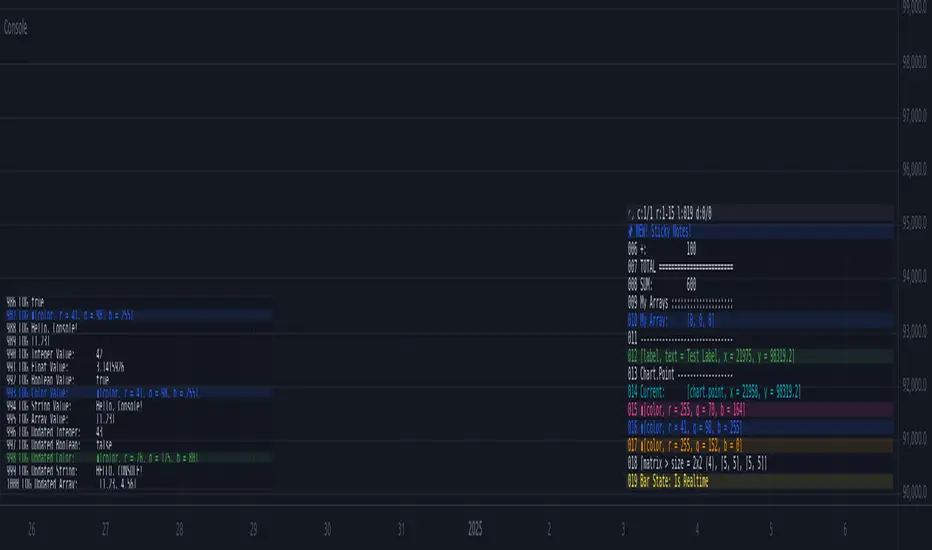
Console📕 Console Library
🔷 Introduction
This script is an adaptation of the classic JavaScript console script. It provides a simple way to display data in a console-like table format for debugging purposes.
While there are many nice console/logger scripts out there, my personal goal was to achieve inline functionality and visual object (label, lines) logging .
🔷 How to Use
◼ 1. Import the Console library into your script:
import cryptolinx/Console/1
- or -
Instead of the library namespace, you can define a custom namespace as alias.
import cryptolinx/Console/1 as c
◼ 2. Create and init a new `` object.
The `init()` method is used to initialize the console object with default settings. It can be used to customize it.
// When using the `var` keyword in a declaration, the logs will act as ever-forwarding.
// Without `var`, the `console` variable will be redeclared every time `bar` is called.
// var console = Console.terminal.new(log_position=position.bottom_left, prefix = '> ', show_no = true)
- or -
If you has set up an alias before.
var console = c.terminal.new().init()
◼ 3. Logging
// inline ✨
array testArray = array.new(3, .0).log(console)
// basic
console.log(testArray)
// inline ✨
var testLabel = label.new(bar_index, close, 'Label Text').log(console)
// basic
console.log(testLabel)
// It is also possible to use `().` for literals ✨.
int a = 100
testCalc = (5 * 100).log(console) + a.log(console) // SUM: 600
console.
.empty()
.log('SUM' + WS + testCalc.tostring())
◼ 4. Visibility
Finally, we need to call the `show()` method to display the logged messages in the console.
console.show(true) // True by default. Simply turn it on or off
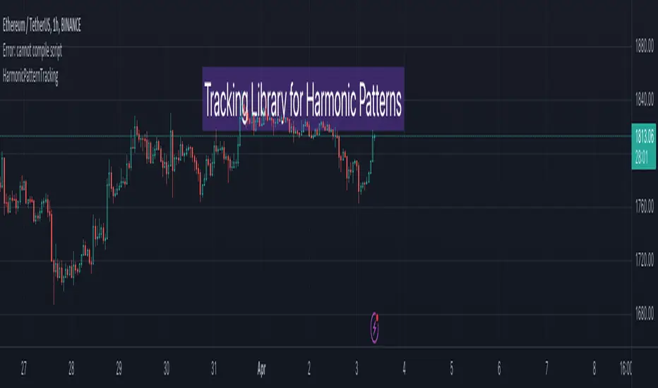
HarmonicPatternTrackingLibrary "HarmonicPatternTracking"
Library contains few data structures and methods for tracking harmonic pattern trades via pinescript.
method draw(this)
Creates and draws HarmonicDrawing object for given HarmonicPattern
Namespace types: HarmonicPattern
Parameters:
this (HarmonicPattern) : HarmonicPattern object
Returns: current HarmonicPattern object
method addTrade(this)
calculates HarmonicTrade and sets trade object for HarmonicPattern
Namespace types: HarmonicPattern
Parameters:
this (HarmonicPattern) : HarmonicPattern object
Returns: bool true if pattern trades are valid, false otherwise
method delete(this)
Deletes drawing objects of HarmonicDrawing
Namespace types: HarmonicDrawing
Parameters:
this (HarmonicDrawing) : HarmonicDrawing object
Returns: current HarmonicDrawing object
method delete(this)
Deletes drawings of harmonic pattern
Namespace types: HarmonicPattern
Parameters:
this (HarmonicPattern) : HarmonicPattern object
Returns: current HarmonicPattern object
HarmonicDrawing
Drawing objects of Harmonic Pattern
Fields:
xa (series line) : xa line
ab (series line) : ab line
bc (series line) : bc line
cd (series line) : cd line
xb (series line) : xb line
bd (series line) : bd line
ac (series line) : ac line
xd (series line) : xd line
x (series label) : label for pivot x
a (series label) : label for pivot a
b (series label) : label for pivot b
c (series label) : label for pivot c
d (series label) : label for pivot d
xabRatio (series label) : label for XAB Ratio
abcRatio (series label) : label for ABC Ratio
bcdRatio (series label) : label for BCD Ratio
xadRatio (series label) : label for XAD Ratio
HarmonicTrade
Trade tracking parameters of Harmonic Patterns
Fields:
initialEntry (series float) : initial entry when pattern first formed.
entry (series float) : trailed entry price.
initialStop (series float) : initial stop when trade first entered.
stop (series float) : current stop updated as per trailing rules.
target1 (series float) : First target value
target2 (series float) : Second target value
target3 (series float) : Third target value
target4 (series float) : Fourth target value
status (series int) : Trade status referenced as integer
retouch (series bool) : Flag to show if the price retouched after entry
HarmonicProperties
Display and trade calculation properties for Harmonic Patterns
Fields:
fillMajorTriangles (series bool) : Display property used for using linefill for harmonic major triangles
fillMinorTriangles (series bool) : Display property used for using linefill for harmonic minor triangles
majorFillTransparency (series int) : transparency setting for major triangles
minorFillTransparency (series int) : transparency setting for minor triangles
showXABCD (series bool) : Display XABCD pivot labels
lblSizePivots (series string) : Pivot label size
showRatios (series bool) : Display Ratio labels
useLogScaleForScan (series bool) : Use log scale to determine fib ratios for pattern scanning
useLogScaleForTargets (series bool) : Use log scale to determine fib ratios for target calculation
base (series string) : base on which calculation of stop/targets are made.
entryRatio (series float) : fib ratio to calculate entry
stopRatio (series float) : fib ratio to calculate initial stop
target1Ratio (series float) : fib ratio to calculate first target
target2Ratio (series float) : fib ratio to calculate second target
target3Ratio (series float) : fib ratio to calculate third target
target4Ratio (series float) : fib ratio to calculate fourth target
HarmonicPattern
Harmonic pattern object to track entire pattern trade life cycle
Fields:
id (series int) : Pattern Id
dir (series int) : pattern direction
x (series float) : X Pivot
a (series float) : A Pivot
b (series float) : B Pivot
c (series float) : C Pivot
d (series float) : D Pivot
xBar (series int) : Bar index of X Pivot
aBar (series int) : Bar index of A Pivot
bBar (series int) : Bar index of B Pivot
cBar (series int) : Bar index of C Pivot
dBar (series int) : Bar index of D Pivot
przStart (series float) : Start of PRZ range
przEnd (series float) : End of PRZ range
patterns (bool ) : array representing the patterns
patternLabel (series string) : string representation of list of patterns
patternColor (series color) : color assigned to pattern
properties (HarmonicProperties) : HarmonicProperties object containing display and calculation properties
trade (HarmonicTrade) : HarmonicTrade object to track trades
drawing (HarmonicDrawing) : HarmonicDrawing object to manage drawings
OHLC📕 LIBRARY OHLC
🔷 Introduction
This library is a custom library designed to work with real-time bars. It allows to easily calculate OHLC values for any source.
Personally, I use this library to accurately display the highest and lowest values on visual indicators such as my progress bars.
🔷 How to Use
◼ 1. Import the OHLC library into your TradingView script:
import cryptolinx/OHLC/1
- or -
Instead of the library namespace, you can define a custom namespace as alias.
import cryptolinx/OHLC/1 as src
◼ 2. Create a new OHLC source using the `new()` function.
varip mySrc = OHLC.new() // It is required to use the `varip` keyword to init your ``
- or -
If you has set up an alias before.
varip mySrc = src.new()
===
In that case, your `` needs to be `na`, define your object like that
varip mySrc = na
◼ 3. Call the `hydrateOHLC()` method on your OHLC source to update its values:
Basic
float rsi = ta.rsi(close, 14)
mySrc.hydrateOHLC(rsi)
- or -
Inline
rsi = ta.rsi(close, 14).hydrateOHLC(mySrc)
◼ 4. The data is accessible under their corresponding names.
mySrc.open
mySrc.high
mySrc.low
mySrc.close
🔷 Note: This library only works with real-time bars and will not work with historical bars.

MarkovChainLibrary "MarkovChain"
Generic Markov Chain type functions.
---
A Markov chain or Markov process is a stochastic model describing a sequence of possible events in which the
probability of each event depends only on the state attained in the previous event.
---
reference:
Understanding Markov Chains, Examples and Applications. Second Edition. Book by Nicolas Privault.
en.wikipedia.org
www.geeksforgeeks.org
towardsdatascience.com
github.com
stats.stackexchange.com
timeseriesreasoning.com
www.ris-ai.com
github.com
gist.github.com
github.com
gist.github.com
writings.stephenwolfram.com
kevingal.com
towardsdatascience.com
spedygiorgio.github.io
github.com
www.projectrhea.org
method to_string(this)
Translate a Markov Chain object to a string format.
Namespace types: MC
Parameters:
this (MC) : `MC` . Markov Chain object.
Returns: string
method to_table(this, position, text_color, text_size)
Namespace types: MC
Parameters:
this (MC)
position (string)
text_color (color)
text_size (string)
method create_transition_matrix(this)
Namespace types: MC
Parameters:
this (MC)
method generate_transition_matrix(this)
Namespace types: MC
Parameters:
this (MC)
new_chain(states, name)
Parameters:
states (state )
name (string)
from_data(data, name)
Parameters:
data (string )
name (string)
method probability_at_step(this, target_step)
Namespace types: MC
Parameters:
this (MC)
target_step (int)
method state_at_step(this, start_state, target_state, target_step)
Namespace types: MC
Parameters:
this (MC)
start_state (int)
target_state (int)
target_step (int)
method forward(this, obs)
Namespace types: HMC
Parameters:
this (HMC)
obs (int )
method backward(this, obs)
Namespace types: HMC
Parameters:
this (HMC)
obs (int )
method viterbi(this, observations)
Namespace types: HMC
Parameters:
this (HMC)
observations (int )
method baumwelch(this, observations)
Namespace types: HMC
Parameters:
this (HMC)
observations (int )
Node
Target node.
Fields:
index (series int) : . Key index of the node.
probability (series float) : . Probability rate of activation.
state
State reference.
Fields:
name (series string) : . Name of the state.
index (series int) : . Key index of the state.
target_nodes (Node ) : . List of index references and probabilities to target states.
MC
Markov Chain reference object.
Fields:
name (series string) : . Name of the chain.
states (state ) : . List of state nodes and its name, index, targets and transition probabilities.
size (series int) : . Number of unique states
transitions (matrix) : . Transition matrix
HMC
Hidden Markov Chain reference object.
Fields:
name (series string) : . Name of thehidden chain.
states_hidden (state ) : . List of state nodes and its name, index, targets and transition probabilities.
states_obs (state ) : . List of state nodes and its name, index, targets and transition probabilities.
transitions (matrix) : . Transition matrix
emissions (matrix) : . Emission matrix
initial_distribution (float )

FunctionProbabilityViterbiLibrary "FunctionProbabilityViterbi"
The Viterbi Algorithm calculates the most likely sequence of hidden states *(called Viterbi path)*
that results in a sequence of observed events.
viterbi(observations, transitions, emissions, initial_distribution)
Calculate most probable path in a Markov model.
Parameters:
observations (int ) : array . Observation states data.
transitions (matrix) : matrix . Transition probability table, (HxH, H:Hidden states).
emissions (matrix) : matrix . Emission probability table, (OxH, O:Observed states).
initial_distribution (float ) : array . Initial probability distribution for the hidden states.
Returns: array. Most probable path.

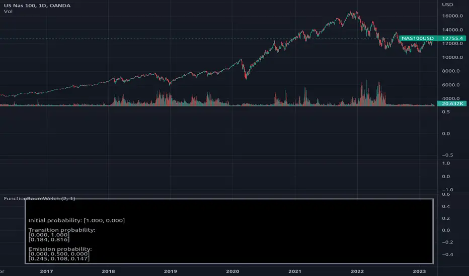
FunctionBaumWelchLibrary "FunctionBaumWelch"
Baum-Welch Algorithm, also known as Forward-Backward Algorithm, uses the well known EM algorithm
to find the maximum likelihood estimate of the parameters of a hidden Markov model given a set of observed
feature vectors.
---
### Function List:
> `forward (array pi, matrix a, matrix b, array obs)`
> `forward (array pi, matrix a, matrix b, array obs, bool scaling)`
> `backward (matrix a, matrix b, array obs)`
> `backward (matrix a, matrix b, array obs, array c)`
> `baumwelch (array observations, int nstates)`
> `baumwelch (array observations, array pi, matrix a, matrix b)`
---
### Reference:
> en.wikipedia.org
> github.com
> en.wikipedia.org
> www.rdocumentation.org
> www.rdocumentation.org
forward(pi, a, b, obs)
Computes forward probabilities for state `X` up to observation at time `k`, is defined as the
probability of observing sequence of observations `e_1 ... e_k` and that the state at time `k` is `X`.
Parameters:
pi (float ) : Initial probabilities.
a (matrix) : Transmissions, hidden transition matrix a or alpha = transition probability matrix of changing
states given a state matrix is size (M x M) where M is number of states.
b (matrix) : Emissions, matrix of observation probabilities b or beta = observation probabilities. Given
state matrix is size (M x O) where M is number of states and O is number of different
possible observations.
obs (int ) : List with actual state observation data.
Returns: - `matrix _alpha`: Forward probabilities. The probabilities are given on a logarithmic scale (natural logarithm). The first
dimension refers to the state and the second dimension to time.
forward(pi, a, b, obs, scaling)
Computes forward probabilities for state `X` up to observation at time `k`, is defined as the
probability of observing sequence of observations `e_1 ... e_k` and that the state at time `k` is `X`.
Parameters:
pi (float ) : Initial probabilities.
a (matrix) : Transmissions, hidden transition matrix a or alpha = transition probability matrix of changing
states given a state matrix is size (M x M) where M is number of states.
b (matrix) : Emissions, matrix of observation probabilities b or beta = observation probabilities. Given
state matrix is size (M x O) where M is number of states and O is number of different
possible observations.
obs (int ) : List with actual state observation data.
scaling (bool) : Normalize `alpha` scale.
Returns: - #### Tuple with:
> - `matrix _alpha`: Forward probabilities. The probabilities are given on a logarithmic scale (natural logarithm). The first
dimension refers to the state and the second dimension to time.
> - `array _c`: Array with normalization scale.
backward(a, b, obs)
Computes backward probabilities for state `X` and observation at time `k`, is defined as the probability of observing the sequence of observations `e_k+1, ... , e_n` under the condition that the state at time `k` is `X`.
Parameters:
a (matrix) : Transmissions, hidden transition matrix a or alpha = transition probability matrix of changing states
given a state matrix is size (M x M) where M is number of states
b (matrix) : Emissions, matrix of observation probabilities b or beta = observation probabilities. given state
matrix is size (M x O) where M is number of states and O is number of different possible observations
obs (int ) : Array with actual state observation data.
Returns: - `matrix _beta`: Backward probabilities. The probabilities are given on a logarithmic scale (natural logarithm). The first dimension refers to the state and the second dimension to time.
backward(a, b, obs, c)
Computes backward probabilities for state `X` and observation at time `k`, is defined as the probability of observing the sequence of observations `e_k+1, ... , e_n` under the condition that the state at time `k` is `X`.
Parameters:
a (matrix) : Transmissions, hidden transition matrix a or alpha = transition probability matrix of changing states
given a state matrix is size (M x M) where M is number of states
b (matrix) : Emissions, matrix of observation probabilities b or beta = observation probabilities. given state
matrix is size (M x O) where M is number of states and O is number of different possible observations
obs (int ) : Array with actual state observation data.
c (float ) : Array with Normalization scaling coefficients.
Returns: - `matrix _beta`: Backward probabilities. The probabilities are given on a logarithmic scale (natural logarithm). The first dimension refers to the state and the second dimension to time.
baumwelch(observations, nstates)
**(Random Initialization)** Baum–Welch algorithm is a special case of the expectation–maximization algorithm used to find the
unknown parameters of a hidden Markov model (HMM). It makes use of the forward-backward algorithm
to compute the statistics for the expectation step.
Parameters:
observations (int ) : List of observed states.
nstates (int)
Returns: - #### Tuple with:
> - `array _pi`: Initial probability distribution.
> - `matrix _a`: Transition probability matrix.
> - `matrix _b`: Emission probability matrix.
---
requires: `import RicardoSantos/WIPTensor/2 as Tensor`
baumwelch(observations, pi, a, b)
Baum–Welch algorithm is a special case of the expectation–maximization algorithm used to find the
unknown parameters of a hidden Markov model (HMM). It makes use of the forward-backward algorithm
to compute the statistics for the expectation step.
Parameters:
observations (int ) : List of observed states.
pi (float ) : Initial probaility distribution.
a (matrix) : Transmissions, hidden transition matrix a or alpha = transition probability matrix of changing states
given a state matrix is size (M x M) where M is number of states
b (matrix) : Emissions, matrix of observation probabilities b or beta = observation probabilities. given state
matrix is size (M x O) where M is number of states and O is number of different possible observations
Returns: - #### Tuple with:
> - `array _pi`: Initial probability distribution.
> - `matrix _a`: Transition probability matrix.
> - `matrix _b`: Emission probability matrix.
---
requires: `import RicardoSantos/WIPTensor/2 as Tensor`
MyLibraryLibrary "MyLibrary"
TODO: add library description here
fun(x)
TODO: add function description here
Parameters:
x (float) : TODO: add parameter x description here
Returns: TODO: add what function returns
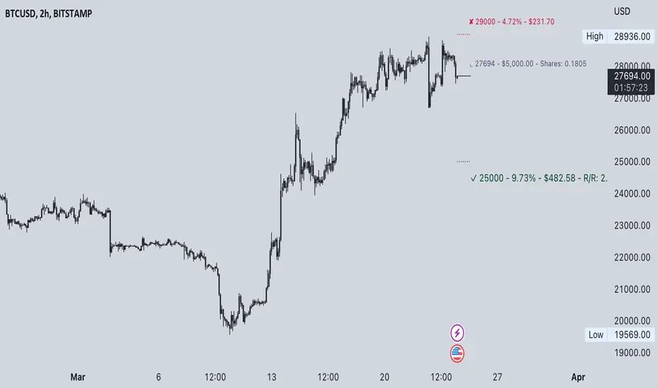
Commission-aware Trade LabelsCommission-aware Trade Labels
Description:
This library provides an easy way to visualize take-profit and stop-loss levels on your chart, taking into account trading commissions. The library calculates and displays the net profit or loss, along with other useful information such as risk/reward ratio, shares, and position size.
Features:
Configurable take-profit and stop-loss prices or percentages.
Set entry amount or shares.
Calculates and displays the risk/reward ratio.
Shows net profit or loss, considering trading commissions.
Customizable label appearance.
Usage:
Add the script to your chart.
Create an Order object for take-profit and stop-loss with desired configurations.
Call target_label() and stop_label() methods for each order object.
Example:
target_order = Order.new(take_profit_price=27483, stop_loss_price=28000, shares=0.2)
stop_order = Order.new(stop_loss_price=29000, shares=1)
target_order.target_label()
stop_order.stop_label()
This script is a powerful tool for visualizing your trading strategy's performance and helps you make better-informed decisions by considering trading commissions in your profit and loss calculations.
Library "tradelabels"
entry_price(this)
Parameters:
this : Order object
@return entry_price
take_profit_price(this)
Parameters:
this : Order object
@return take_profit_price
stop_loss_price(this)
Parameters:
this : Order object
@return stop_loss_price
is_long(this)
Parameters:
this : Order object
@return entry_price
is_short(this)
Parameters:
this : Order object
@return entry_price
percent_to_target(this, target)
Parameters:
this : Order object
target : Target price
@return percent
risk_reward(this)
Parameters:
this : Order object
@return risk_reward_ratio
shares(this)
Parameters:
this : Order object
@return shares
position_size(this)
Parameters:
this : Order object
@return position_size
commission_cost(this, target_price)
Parameters:
this : Order object
@return commission_cost
target_price
net_result(this, target_price)
Parameters:
this : Order object
target_price : The target price to calculate net result for (either take_profit_price or stop_loss_price)
@return net_result
create_take_profit_label(this, prefix, size, offset_x, bg_color, text_color)
Parameters:
this
prefix
size
offset_x
bg_color
text_color
create_stop_loss_label(this, prefix, size, offset_x, bg_color, text_color)
Parameters:
this
prefix
size
offset_x
bg_color
text_color
create_entry_label(this, prefix, size, offset_x, bg_color, text_color)
Parameters:
this
prefix
size
offset_x
bg_color
text_color
create_line(this, target_price, line_color, offset_x, line_style, line_width, draw_entry_line)
Parameters:
this
target_price
line_color
offset_x
line_style
line_width
draw_entry_line
Order
Order
Fields:
entry_price : Entry price
stop_loss_price : Stop loss price
stop_loss_percent : Stop loss percent, default 2%
take_profit_price : Take profit price
take_profit_percent : Take profit percent, default 6%
entry_amount : Entry amount, default 5000$
shares : Shares
commission : Commission, default 0.04%
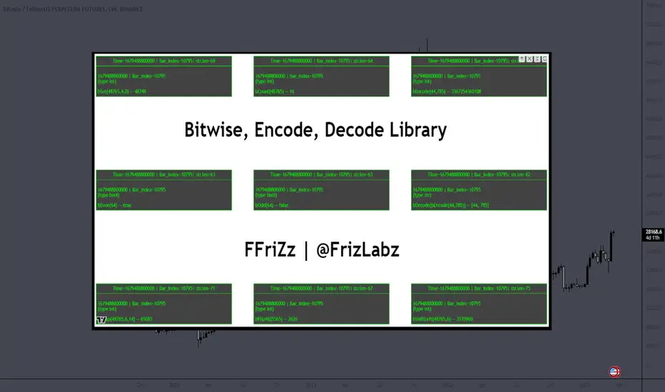
Bitwise, Encode, DecodeLibrary "Bitwise, Encode, Decode"
Bitwise, Encode, Decode, and more Library
docs()
Hover-Over Documentation for inside Text Editor
bAnd(a, b)
Returns the bitwise AND of two integers
Parameters:
a : `int` - The first integer
b : `int` - The second integer
Returns: `int` - The bitwise AND of the two integers
bOr(a, b)
Performs a bitwise OR operation on two integers.
Parameters:
a : `int` - The first integer.
b : `int` - The second integer.
Returns: `int` - The result of the bitwise OR operation.
bXor(a, b)
Performs a bitwise Xor operation on two integers.
Parameters:
a : `int` - The first integer.
b : `int` - The second integer.
Returns: `int` - The result of the bitwise Xor operation.
bNot(n)
Performs a bitwise NOT operation on an integer.
Parameters:
n : `int` - The integer to perform the bitwise NOT operation on.
Returns: `int` - The result of the bitwise NOT operation.
bShiftLeft(n, step)
Performs a bitwise left shift operation on an integer.
Parameters:
n : `int` - The integer to perform the bitwise left shift operation on.
step : `int` - The number of positions to shift the bits to the left.
Returns: `int` - The result of the bitwise left shift operation.
bShiftRight(n, step)
Performs a bitwise right shift operation on an integer.
Parameters:
n : `int` - The integer to perform the bitwise right shift operation on.
step : `int` - The number of bits to shift by.
Returns: `int` - The result of the bitwise right shift operation.
bRotateLeft(n, step)
Performs a bitwise right shift operation on an integer.
Parameters:
n : `int` - The int to perform the bitwise Left rotation on the bits.
step : `int` - The number of bits to shift by.
Returns: `int`- The result of the bitwise right shift operation.
bRotateRight(n, step)
Performs a bitwise right shift operation on an integer.
Parameters:
n : `int` - The int to perform the bitwise Right rotation on the bits.
step : `int` - The number of bits to shift by.
Returns: `int` - The result of the bitwise right shift operation.
bSetCheck(n, pos)
Checks if the bit at the given position is set to 1.
Parameters:
n : `int` - The integer to check.
pos : `int` - The position of the bit to check.
Returns: `bool` - True if the bit is set to 1, False otherwise.
bClear(n, pos)
Clears a particular bit of an integer (changes from 1 to 0) passes if bit at pos is 0.
Parameters:
n : `int` - The integer to clear a bit from.
pos : `int` - The zero-based index of the bit to clear.
Returns: `int` - The result of clearing the specified bit.
bFlip0s(n)
Flips all 0 bits in the number to 1.
Parameters:
n : `int` - The integer to flip the bits of.
Returns: `int` - The result of flipping all 0 bits in the number.
bFlip1s(n)
Flips all 1 bits in the number to 0.
Parameters:
n : `int` - The integer to flip the bits of.
Returns: `int` - The result of flipping all 1 bits in the number.
bFlipAll(n)
Flips all bits in the number.
Parameters:
n : `int` - The integer to flip the bits of.
Returns: `int` - The result of flipping all bits in the number.
bSet(n, pos, newBit)
Changes the value of the bit at the given position.
Parameters:
n : `int` - The integer to modify.
pos : `int` - The position of the bit to change.
newBit : `int` - na = flips bit at pos reguardless 1 or 0 | The new value of the bit (0 or 1).
Returns: `int` - The modified integer.
changeDigit(n, pos, newDigit)
Changes the value of the digit at the given position.
Parameters:
n : `int` - The integer to modify.
pos : `int` - The position of the digit to change.
newDigit : `int` - The new value of the digit (0-9).
Returns: `int` - The modified integer.
bSwap(n, i, j)
Switch the position of 2 bits of an int
Parameters:
n : `int` - int to manipulate
i : `int` - bit pos to switch with j
j : `int` - bit pos to switch with i
Returns: `int` - new int with bits switched
bPalindrome(n)
Checks to see if the binary form is a Palindrome (reads the same left to right and vice versa)
Parameters:
n : `int` - int to check
Returns: `bool` - result of check
bEven(n)
Checks if n is Even
Parameters:
n : `int` - The integer to check.
Returns: `bool` - result.
bOdd(n)
checks if n is Even if not even Odd
Parameters:
n : `int` - The integer to check.
Returns: `bool` - result.
bPowerOfTwo(n)
Checks if n is a Power of 2.
Parameters:
n : `int` - number to check.
Returns: `bool` - result.
bCount(n, to_count)
Counts the number of bits that are equal to 1 in an integer.
Parameters:
n : `int` - The integer to count the bits in.
to_count `string` - the bits to count
Returns: `int` - The number of bits that are equal to 1 in n.
GCD(a, b)
Finds the greatest common divisor (GCD) of two numbers.
Parameters:
a : `int` - The first number.
b : `int` - The second number.
Returns: `int` - The GCD of a and b.
LCM(a, b)
Finds the least common multiple (LCM) of two integers.
Parameters:
a : `int` - The first integer.
b : `int` - The second integer.
Returns: `int` - The LCM of a and b.
aLCM(nums)
Finds the LCM of an array of integers.
Parameters:
nums : `int ` - The list of integers.
Returns: `int` - The LCM of the integers in nums.
adjustedLCM(nums, LCM)
adjust an array of integers to Least Common Multiple (LCM)
Parameters:
nums : `int ` - The first integer
LCM : `int` - The second integer
Returns: `int ` - array of ints with LCM
charAt(str, pos)
gets a Char at a given position.
Parameters:
str : `string` - string to pull char from.
pos : `int` - pos to get char from string (left to right index).
Returns: `string` - char from pos of string or "" if pos is not within index range
decimalToBinary(num)
Converts a decimal number to binary
Parameters:
num : `int` - The decimal number to convert to binary
Returns: `string` - The binary representation of the decimal number
decimalToBinary(num, to_binary_int)
Converts a decimal number to binary
Parameters:
num : `int` - The decimal number to convert to binary
to_binary_int : `bool` - bool to convert to int or to string (true for int, false for string)
Returns: `string` - The binary representation of the decimal number
binaryToDecimal(binary)
Converts a binary number to decimal
Parameters:
binary : `string` - The binary number to convert to decimal
Returns: `int` - The decimal representation of the binary number
decimal_len(n)
way of finding decimal length using arithmetic
Parameters:
n `float` - floating decimal point to get length of.
Returns: `int` - number of decimal places
int_len(n)
way of finding number length using arithmetic
Parameters:
n : `int`- value to find length of number
Returns: `int` - lenth of nunber i.e. 23 == 2
float_decimal_to_whole(n)
Converts a float decimal number to an integer `0.365 to 365`.
Parameters:
n : `string` - The decimal number represented as a string.
Returns: `int` - The integer obtained by removing the decimal point and leading zeroes from s.
fractional_part(x)
Returns the fractional part of a float.
Parameters:
x : `float` - The float to get the fractional part of.
Returns: `float` - The fractional part of the float.
form_decimal(a, b, zero_fix)
helper to form 2 ints into 1 float seperated by the decimal
Parameters:
a : `int` - a int
b : `int` - b int
zero_fix : `bool` - fix for trailing zeros being truncated when converting to float
Returns: ` ` - float = float decimal of ints | string = string version of b for future use to ref length
bEncode(n1, n2)
Encodes two numbers into one using bit OR. (fastest)
Parameters:
n1 : `int` - The first number to Encodes.
n2 : `int` - The second number to Encodes.
Returns: `int` - The result of combining the two numbers using bit OR.
bDecode(n)
Decodes an integer created by the bCombine function.(fastest)
Parameters:
n : `int` - The integer to decode.
Returns: ` ` - A tuple containing the two decoded components of the integer.
Encode(a, b)
Encodes by seperating ints into left and right of decimal float
Parameters:
a : `int` - a int
b : `int` - b int
Returns: `float` - new float of encoded ints one on left of decimal point one on right
Decode(encoded)
Decodes float of 2 ints seperated by decimal point
Parameters:
encoded : `float` - the encoded float value
Returns: ` ` - tuple of the 2 ints from encoded float
encode_heavy(a, b)
Encodes by combining numbers and tracking size in the
decimal of a floating number (slowest)
Parameters:
a : `int` - a int
b : `int` - b int
Returns: `float` - new decimal of encoded ints
decode_heavy(encoded)
Decodes encoded float that tracks size of ints in float decimal
Parameters:
encoded : `float` - encoded float
Returns: ` ` - tuple of decoded ints
decimal of float (slowest)
Parameters:
encoded : `float` - the encoded float value
Returns: ` ` - tuple of the 2 ints from encoded float
Bitwise, Encode, Decode Docs
In the documentation you may notice the word decimal
not used as normal this is because when referring to
binary a decimal number is a number that
can be represented with base 10 numbers 0-9
(the wiki below explains better)
A rule of thumb for the two integers being
encoded it to keep both numbers
less than 65535 this is because anything lower uses 16 bits or less
this will maintain 100% accuracy when decoding
although it is possible to do numbers up to 2147483645 with
this library doesnt seem useful enough
to explain or demonstrate.
The functions provided work within this 32-bit range,
where the highest number is all 1s and
the lowest number is all 0s. These functions were created
to overcome the lack of built-in bitwise functions in Pinescript.
By combining two integers into a single number,
the code can access both values i.e when
indexing only one array index
for a matrices row/column, thus improving execution time.
This technique can be applied to various coding
scenarios to enhance performance.
Bitwise functions are a way to use integers in binary form
that can be used to speed up several different processes
most languages have operators to perform these function such as
`<<, >>, &, ^, |, ~`
en.wikipedia.org
DataChartLibrary "DataChart"
Library to plot scatterplot or heatmaps for your own set of data samples
draw(this)
draw contents of the chart object
Parameters:
this : Chart object
Returns: current chart object
init(this)
Initialize Chart object.
Parameters:
this : Chart object to be initialized
Returns: current chart object
addSample(this, sample, trigger)
Add sample data to chart using Sample object
Parameters:
this : Chart object
sample : Sample object containing sample x and y values to be plotted
trigger : Samples are added to chart only if trigger is set to true. Default value is true
Returns: current chart object
addSample(this, x, y, trigger)
Add sample data to chart using x and y values
Parameters:
this : Chart object
x : x value of sample data
y : y value of sample data
trigger : Samples are added to chart only if trigger is set to true. Default value is true
Returns: current chart object
addPriceSample(this, priceSampleData, config)
Add price sample data - special type of sample designed to measure price displacements of events
Parameters:
this : Chart object
priceSampleData : PriceSampleData object containing event driven displacement data of x and y
config : PriceSampleConfig object containing configurations for deriving x and y from priceSampleData
Returns: current chart object
Sample
Sample data for chart
Fields:
xValue : x value of the sample data
yValue : y value of the sample data
ChartProperties
Properties of plotting chart
Fields:
title : Title of the chart
suffix : Suffix for values. It can be used to reference 10X or 4% etc. Used only if format is not format.percent
matrixSize : size of the matrix used for plotting
chartType : Can be either scatterplot or heatmap. Default is scatterplot
outliersStart : Indicates the percentile of data to filter out from the starting point to get rid of outliers
outliersEnd : Indicates the percentile of data to filter out from the ending point to get rid of outliers.
backgroundColor
plotColor : color of plots on the chart. Default is color.yellow. Only used for scatterplot type
heatmapColor : color of heatmaps on the chart. Default is color.red. Only used for heatmap type
borderColor : border color of the chart table. Default is color.yellow.
plotSize : size of scatter plots. Default is size.large
format : data representation format in tooltips. Use mintick.percent if measuring any data in terms of percent. Else, use format.mintick
showCounters : display counters which shows totals on each quadrants. These are single cell tables at the corners displaying number of occurences on each quadrant.
showTitle : display title at the top center. Uses the title string set in the properties
counterBackground : background color of counter table cells. Default is color.teal
counterTextColor : text color of counter table cells. Default is color.white
counterTextSize : size of counter table cells. Default is size.large
titleBackground : background color of chart title. Default is color.maroon
titleTextColor : text color of the chart title. Default is color.white
titleTextSize : text size of the title cell. Default is size.large
addOutliersToBorder : If set, instead of removing the outliers, it will be added to the border cells.
useCommonScale : Use common scale for both x and y. If not selected, different scales are calculated based on range of x and y values from samples. Default is set to false.
plotchar : scatter plot character. Default is set to ascii bullet.
ChartDrawing
Chart drawing objects collection
Fields:
properties : ChartProperties object which determines the type and characteristics of chart being plotted
titleTable : table containing title of the chart.
mainTable : table containing plots or heatmaps.
quadrantTables : Array of tables containing counters of all 4 quandrants
Chart
Chart type which contains all the information of chart being plotted
Fields:
properties : ChartProperties object which determines the type and characteristics of chart being plotted
samples : Array of Sample objects collected over period of time for plotting on chart.
displacements : Array containing displacement values. Both x and y values
displacementX : Array containing only X displacement values.
displacementY : Array containing only Y displacement values.
drawing : ChartDrawing object which contains all the drawing elements
PriceSampleConfig
Configs used for adding specific type of samples called PriceSamples
Fields:
duration : impact duration for which price displacement samples are calculated.
useAtrReference : Default is true. If set to true, price is measured in terms of Atr. Else is measured in terms of percentage of price.
atrLength : atrLength to be used for measuring the price based on ATR. Used only if useAtrReference is set to true.
PriceSampleData
Special type of sample called price sample. Can be used instead of basic Sample type
Fields:
trigger : consider sample only if trigger is set to true. Default is true.
source : Price source. Default is close
highSource : High price source. Default is high
lowSource : Low price source. Default is low
tr : True range value. Default is ta.tr

Feature ScalingLibrary "Feature_Scaling"
FS: This library helps you scale your data to certain ranges or standarize, normalize, unit scale or min-max scale your data in your prefered way. Mostly used for normalization purposes.
minmaxscale(source, min, max, length)
minmaxscale: Min-max normalization scales your data to set minimum and maximum range
Parameters:
source
min
max
length
Returns: res: Data scaled to the set minimum and maximum range
meanscale(source, length)
meanscale: Mean normalization of your data
Parameters:
source
length
Returns: res: Mean normalization result of the source
standarize(source, length, biased)
standarize: Standarization of your data
Parameters:
source
length
biased
Returns: res: Standarized data
unitlength(source, length)
unitlength: Scales your data into overall unit length
Parameters:
source
length
Returns: res: Your data scaled to the unit length
TableBuilderLibrary "TableBuilder"
A helper library to make it simpler to create tables in pinescript
This is a simple table building library that I created because I personally feel that the built-in table building method is too verbose. It features chaining methods and variable arguments.
There are many features that are lacking because the implementation is early, and there may be antipatterns because I am not familiar with the runtime behavior like pinescript. If you have any comments on code improvements or features you want, please comment :D

SILLibrary "SIL"
mean_src(x, y)
calculates moving average : x is the source of price (OHLC) & y = the lookback period
Parameters:
x
y
stan_dev(x, y, z)
calculates standard deviation, x = source of price (OHLC), y = the average lookback, z = average given prior two float and intger inputs, call the f_avg_src() function in f_stan_dev()
Parameters:
x
y
z
vawma(x, y)
calculates volume weighted moving average, x = source of price (OHLC), y = loookback period
Parameters:
x
y
gethurst(x, y, z)
calculates the Hurst Exponent and Hurst Exponent average, x = source of price (OHLC), y = lookback period for Hurst Exponent Calculation, z = lookback period for average Hurst Exponent
Parameters:
x
y
z

libKageMiscLibrary "libKageMisc"
Kage's Miscelaneous library
print(_value)
Print a numerical value in a label at last historical bar.
Parameters:
_value : (float) The value to be printed.
Returns: Nothing.
barsBackToDate(_year, _month, _day)
Get the number of bars we have to go back to get data from a specific date.
Parameters:
_year : (int) Year of the specific date.
_month : (int) Month of the specific date. Optional. Default = 1.
_day : (int) Day of the specific date. Optional. Default = 1.
Returns: (int) Number of bars to go back until reach the specific date.
bodySize(_index)
Calculates the size of the bar's body.
Parameters:
_index : (simple int) The historical index of the bar. Optional. Default = 0.
Returns: (float) The size of the bar's body in price units.
shadowSize(_direction)
Size of the current bar shadow. Either "top" or "bottom".
Parameters:
_direction : (string) Direction of the desired shadow.
Returns: (float) The size of the chosen bar's shadow in price units.
shadowBodyRatio(_direction)
Proportion of current bar shadow to the bar size
Parameters:
_direction : (string) Direction of the desired shadow.
Returns: (float) Ratio of the shadow size per body size.
bodyCloseRatio(_index)
Proportion of chosen bar body size to the close price
Parameters:
_index : (simple int) The historical index of the bar. Optional. Default = 0.()
Returns: (float) Ratio of the body size per close price.
lastDayOfMonth(_month)
Returns the last day of a month.
Parameters:
_month : (int) Month number.
Returns: (int) The number (28, 30 or 31) of the last day of a given month.
nameOfMonth(_month)
Return the short name of a month.
Parameters:
_month : (int) Month number.
Returns: (string) The short name ("Jan", "Feb"...) of a given month.
pl(_initialValue, _finalValue)
Calculate Profit/Loss between two values.
Parameters:
_initialValue : (float) Initial value.
_finalValue : (float) Final value = Initial value + delta.
Returns: (float) Profit/Loss as a percentual change.
gma(_Type, _Source, _Length)
Generalist Moving Average (GMA).
Parameters:
_Type : (string) Type of average to be used. Either "EMA", "HMA", "RMA", "SMA", "SWMA", "WMA" or "VWMA".
_Source : (series float) Series of values to process.
_Length : (simple int) Number of bars (length).
Returns: (float) The value of the chosen moving average.
xFormat(_percentValue, _minXFactor)
Transform a percentual value in a X Factor value.
Parameters:
_percentValue : (float) Percentual value to be transformed.
_minXFactor : (float) Minimum X Factor to that the conversion occurs. Optional. Default = 10.
Returns: (string) A formated string.
isLong()
Check if the open trade direction is long.
Returns: (bool) True if the open position is long.
isShort()
Check if the open trade direction is short.
Returns: (bool) True if the open position is short.
lastPrice()
Returns the entry price of the last openned trade.
Returns: (float) The last entry price.
barsSinceLastEntry()
Returns the number of bars since last trade was oppened.
Returns: (series int)
getBotNameFrosty()
Return the name of the FrostyBot Bot.
Returns: (string) A string containing the name.
getBotNameZig()
Return the name of the FrostyBot Bot.
Returns: (string) A string containing the name.
getTicksValue(_currencyValue)
Converts currency value to ticks
Parameters:
_currencyValue : (float) Value to be converted.
Returns: (float) Value converted to minticks.
getSymbol(_botName, _botCustomSymbol)
Formats the symbol string to be used with a bot
Parameters:
_botName : (string) Bot name constant. Either BOT_NAME_FROSTY or BOT_NAME_ZIG. Optional. Default is empty string.
_botCustomSymbol : (string) Custom string. Optional. Default is empy string.
Returns: (string) A string containing the symbol for the bot. If all arguments are empty, the current symbol is returned in Binance format.
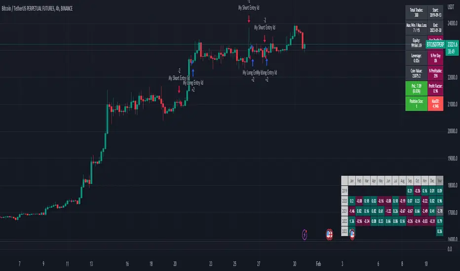
showProfitLossBoard()
Calculates and shows a board of Profit/Loss through the years.
Returns: Nothing.
Liquidation_linesLibrary "Liquidationline"
f_calculateLeverage(_leverage, _maintainance, _value, _direction)
Parameters:
_leverage
_maintainance
_value
_direction
f_liqline_update(_Liqui_Line, _killonlowhigh)
Parameters:
_Liqui_Line
_killonlowhigh
f_liqline_draw(_Liqui_Line, _priceorliq)
Parameters:
_Liqui_Line
_priceorliq
f_liqline_add(_Liqui_Line, linetoadd, _limit)
Parameters:
_Liqui_Line
linetoadd
_limit
Liquidationline
Fields:
creationtime
stoptime
price
leverage
maintainance
line_active
line_color
line_thickness
line_style
line_direction
line_finished
text_active
text_size
text_color
this library can draw typical liquidation lines, which can be called e.g. by indicator signals
You can see the default implementation in the lower part of the code, starting with RUNTIME
Don't forget to increase max lines to 500 in your script.
It can look like this screenshot here, with only minor changes to your executing script.
The base is the same

DistributionsLibrary "Distributions"
Library with price distribution zones calculation helpers.
Based on research from "Trading Systems and Methods, 5th Edition" by Perry J. Kaufman
getZones(h, l, c, window)
Returns price distribution zones based on HLC and for some period
Parameters:
h : high price
l : low price
c : close price
window : period to calculate distributions
Returns: tuple of 5 price zones in descent order, from highest to lowest

PerformanceTableLibrary "PerformanceTable"
TODO: add library description here
This library was created as a library because adding a performance table to an existing strategy script made the strategy script lengthy and inconvenient to manage.
The monthly table script referenced @QuantNomad's code.
The performance table script referenced @myncrypto's code.
To use, copy and paste the code below at the bottom of the strategy script you are using, and the table for strategy performance will be displayed on a chart.
//------------Copy & Paste --------------------------------------//
import Cube_Lee/PerformanceTable/1 as PT
PT = input.bool(true, "Show Performance Table", tooltip = "전략의 성과를 우측상단에 테이블로 표시합니다.", group = "Performance Table")
MT = input.bool(true, "Show Monthly Table", tooltip = "전략의 월별 수익률을 우측하단에 테이블로 표시합니다.", group = "Performance Table")
if PT
PT.PerformanceTable()
if MT
PT.MonthlyTable()
//------------Copy & Paste---------------------------------------//
PerformanceTable()
MonthlyTable()
MLExtensionsLibrary "MLExtensions"
normalizeDeriv(src, quadraticMeanLength)
Returns the smoothed hyperbolic tangent of the input series.
Parameters:
src : The input series (i.e., the first-order derivative for price).
quadraticMeanLength : The length of the quadratic mean (RMS).
Returns: nDeriv The normalized derivative of the input series.
normalize(src, min, max)
Rescales a source value with an unbounded range to a target range.
Parameters:
src : The input series
min : The minimum value of the unbounded range
max : The maximum value of the unbounded range
Returns: The normalized series
rescale(src, oldMin, oldMax, newMin, newMax)
Rescales a source value with a bounded range to anther bounded range
Parameters:
src : The input series
oldMin : The minimum value of the range to rescale from
oldMax : The maximum value of the range to rescale from
newMin : The minimum value of the range to rescale to
newMax : The maximum value of the range to rescale to
Returns: The rescaled series
color_green(prediction)
Assigns varying shades of the color green based on the KNN classification
Parameters:
prediction : Value (int|float) of the prediction
Returns: color
color_red(prediction)
Assigns varying shades of the color red based on the KNN classification
Parameters:
prediction : Value of the prediction
Returns: color
tanh(src)
Returns the the hyperbolic tangent of the input series. The sigmoid-like hyperbolic tangent function is used to compress the input to a value between -1 and 1.
Parameters:
src : The input series (i.e., the normalized derivative).
Returns: tanh The hyperbolic tangent of the input series.
dualPoleFilter(src, lookback)
Returns the smoothed hyperbolic tangent of the input series.
Parameters:
src : The input series (i.e., the hyperbolic tangent).
lookback : The lookback window for the smoothing.
Returns: filter The smoothed hyperbolic tangent of the input series.
tanhTransform(src, smoothingFrequency, quadraticMeanLength)
Returns the tanh transform of the input series.
Parameters:
src : The input series (i.e., the result of the tanh calculation).
smoothingFrequency
quadraticMeanLength
Returns: signal The smoothed hyperbolic tangent transform of the input series.
n_rsi(src, n1, n2)
Returns the normalized RSI ideal for use in ML algorithms.
Parameters:
src : The input series (i.e., the result of the RSI calculation).
n1 : The length of the RSI.
n2 : The smoothing length of the RSI.
Returns: signal The normalized RSI.
n_cci(src, n1, n2)
Returns the normalized CCI ideal for use in ML algorithms.
Parameters:
src : The input series (i.e., the result of the CCI calculation).
n1 : The length of the CCI.
n2 : The smoothing length of the CCI.
Returns: signal The normalized CCI.
n_wt(src, n1, n2)
Returns the normalized WaveTrend Classic series ideal for use in ML algorithms.
Parameters:
src : The input series (i.e., the result of the WaveTrend Classic calculation).
n1
n2
Returns: signal The normalized WaveTrend Classic series.
n_adx(highSrc, lowSrc, closeSrc, n1)
Returns the normalized ADX ideal for use in ML algorithms.
Parameters:
highSrc : The input series for the high price.
lowSrc : The input series for the low price.
closeSrc : The input series for the close price.
n1 : The length of the ADX.
regime_filter(src, threshold, useRegimeFilter)
Parameters:
src
threshold
useRegimeFilter
filter_adx(src, length, adxThreshold, useAdxFilter)
filter_adx
Parameters:
src : The source series.
length : The length of the ADX.
adxThreshold : The ADX threshold.
useAdxFilter : Whether to use the ADX filter.
Returns: The ADX.
filter_volatility(minLength, maxLength, useVolatilityFilter)
filter_volatility
Parameters:
minLength : The minimum length of the ATR.
maxLength : The maximum length of the ATR.
useVolatilityFilter : Whether to use the volatility filter.
Returns: Boolean indicating whether or not to let the signal pass through the filter.
backtest(high, low, open, startLongTrade, endLongTrade, startShortTrade, endShortTrade, isStopLossHit, maxBarsBackIndex, thisBarIndex)
Performs a basic backtest using the specified parameters and conditions.
Parameters:
high : The input series for the high price.
low : The input series for the low price.
open : The input series for the open price.
startLongTrade : The series of conditions that indicate the start of a long trade.`
endLongTrade : The series of conditions that indicate the end of a long trade.
startShortTrade : The series of conditions that indicate the start of a short trade.
endShortTrade : The series of conditions that indicate the end of a short trade.
isStopLossHit : The stop loss hit indicator.
maxBarsBackIndex : The maximum number of bars to go back in the backtest.
thisBarIndex : The current bar index.
Returns: A tuple containing backtest values
init_table()
init_table()
Returns: tbl The backtest results.
update_table(tbl, tradeStatsHeader, totalTrades, totalWins, totalLosses, winLossRatio, winrate, stopLosses)
update_table(tbl, tradeStats)
Parameters:
tbl : The backtest results table.
tradeStatsHeader : The trade stats header.
totalTrades : The total number of trades.
totalWins : The total number of wins.
totalLosses : The total number of losses.
winLossRatio : The win loss ratio.
winrate : The winrate.
stopLosses : The total number of stop losses.
Returns: Updated backtest results table.

DataCorrelationLibrary "DataCorrelation"
Implementation of functions related to data correlation calculations. Formulas have been transformed in such a way that we avoid running loops and instead make use of time series to gradually build the data we need to perform calculation. This allows the calculations to run on unbound series, and/or higher number of samples
🎲 Simplifying Covariance
Original Formula
//For Sample
Covₓᵧ = ∑ ((xᵢ-x̄)(yᵢ-ȳ)) / (n-1)
//For Population
Covₓᵧ = ∑ ((xᵢ-x̄)(yᵢ-ȳ)) / n
Now, if we look at numerator, this can be simplified as follows
∑ ((xᵢ-x̄)(yᵢ-ȳ))
=> (x₁-x̄)(y₁-ȳ) + (x₂-x̄)(y₂-ȳ) + (x₃-x̄)(y₃-ȳ) ... + (xₙ-x̄)(yₙ-ȳ)
=> (x₁y₁ + x̄ȳ - x₁ȳ - y₁x̄) + (x₂y₂ + x̄ȳ - x₂ȳ - y₂x̄) + (x₃y₃ + x̄ȳ - x₃ȳ - y₃x̄) ... + (xₙyₙ + x̄ȳ - xₙȳ - yₙx̄)
=> (x₁y₁ + x₂y₂ + x₃y₃ ... + xₙyₙ) + (x̄ȳ + x̄ȳ + x̄ȳ ... + x̄ȳ) - (x₁ȳ + x₂ȳ + x₃ȳ ... xₙȳ) - (y₁x̄ + y₂x̄ + y₃x̄ + yₙx̄)
=> ∑xᵢyᵢ + n(x̄ȳ) - ȳ∑xᵢ - x̄∑yᵢ
So, overall formula can be simplified to be used in pine as
//For Sample
Covₓᵧ = (∑xᵢyᵢ + n(x̄ȳ) - ȳ∑xᵢ - x̄∑yᵢ) / (n-1)
//For Population
Covₓᵧ = (∑xᵢyᵢ + n(x̄ȳ) - ȳ∑xᵢ - x̄∑yᵢ) / n
🎲 Simplifying Standard Deviation
Original Formula
//For Sample
σ = √(∑(xᵢ-x̄)² / (n-1))
//For Population
σ = √(∑(xᵢ-x̄)² / n)
Now, if we look at numerator within square root
∑(xᵢ-x̄)²
=> (x₁² + x̄² - 2x₁x̄) + (x₂² + x̄² - 2x₂x̄) + (x₃² + x̄² - 2x₃x̄) ... + (xₙ² + x̄² - 2xₙx̄)
=> (x₁² + x₂² + x₃² ... + xₙ²) + (x̄² + x̄² + x̄² ... + x̄²) - (2x₁x̄ + 2x₂x̄ + 2x₃x̄ ... + 2xₙx̄)
=> ∑xᵢ² + nx̄² - 2x̄∑xᵢ
=> ∑xᵢ² + x̄(nx̄ - 2∑xᵢ)
So, overall formula can be simplified to be used in pine as
//For Sample
σ = √(∑xᵢ² + x̄(nx̄ - 2∑xᵢ) / (n-1))
//For Population
σ = √(∑xᵢ² + x̄(nx̄ - 2∑xᵢ) / n)
🎲 Using BinaryInsertionSort library
Chatterjee Correlation and Spearman Correlation functions make use of BinaryInsertionSort library to speed up sorting. The library in turn implements mechanism to insert values into sorted order so that load on sorting is reduced by higher extent allowing the functions to work on higher sample size.
🎲 Function Documentation
chatterjeeCorrelation(x, y, sampleSize, plotSize)
Calculates chatterjee correlation between two series. Formula is - ξnₓᵧ = 1 - (3 * ∑ |rᵢ₊₁ - rᵢ|)/ (n²-1)
Parameters:
x : First series for which correlation need to be calculated
y : Second series for which correlation need to be calculated
sampleSize : number of samples to be considered for calculattion of correlation. Default is 20000
plotSize : How many historical values need to be plotted on chart.
Returns: float correlation - Chatterjee correlation value if falls within plotSize, else returns na
spearmanCorrelation(x, y, sampleSize, plotSize)
Calculates spearman correlation between two series. Formula is - ρ = 1 - (6∑dᵢ²/n(n²-1))
Parameters:
x : First series for which correlation need to be calculated
y : Second series for which correlation need to be calculated
sampleSize : number of samples to be considered for calculattion of correlation. Default is 20000
plotSize : How many historical values need to be plotted on chart.
Returns: float correlation - Spearman correlation value if falls within plotSize, else returns na
covariance(x, y, include, biased)
Calculates covariance between two series of unbound length. Formula is Covₓᵧ = ∑ ((xᵢ-x̄)(yᵢ-ȳ)) / (n-1) for sample and Covₓᵧ = ∑ ((xᵢ-x̄)(yᵢ-ȳ)) / n for population
Parameters:
x : First series for which covariance need to be calculated
y : Second series for which covariance need to be calculated
include : boolean flag used for selectively including sample
biased : boolean flag representing population covariance instead of sample covariance
Returns: float covariance - covariance of selective samples of two series x, y
stddev(x, include, biased)
Calculates Standard Deviation of a series. Formula is σ = √( ∑(xᵢ-x̄)² / n ) for sample and σ = √( ∑(xᵢ-x̄)² / (n-1) ) for population
Parameters:
x : Series for which Standard Deviation need to be calculated
include : boolean flag used for selectively including sample
biased : boolean flag representing population covariance instead of sample covariance
Returns: float stddev - standard deviation of selective samples of series x
correlation(x, y, include)
Calculates pearson correlation between two series of unbound length. Formula is r = Covₓᵧ / σₓσᵧ
Parameters:
x : First series for which correlation need to be calculated
y : Second series for which correlation need to be calculated
include : boolean flag used for selectively including sample
Returns: float correlation - correlation between selective samples of two series x, y

JeeSauceScriptsLibrary "JeeSauceScripts"
getupdnvol()
GetTotalUpVolume(upvolume)
Parameters:
upvolume
GetTotalDnVolume(downvolume)
Parameters:
downvolume
GetDelta(totalupvolume, totaldownvolume)
Parameters:
totalupvolume
totaldownvolume
GetMaxUpVolume(upvolume)
Parameters:
upvolume
GetMaxDnVolume(downvolume)
Parameters:
downvolume
Getcvd()
Getcvdopen(cvd)
Parameters:
cvd
Getcvdhigh(cvd, maxvolumeup)
Parameters:
cvd
maxvolumeup
Getcvdlow(cvd, maxvolumedown)
Parameters:
cvd
maxvolumedown
Getcvdclose(cvd, delta)
Parameters:
cvd
delta
CombineData(data1, data2, data3, data4, data5, data6)
Parameters:
data1
data2
data3
data4
data5
data6
FindData(data, find)
Parameters:
data
find
